01. Introduction to DP0.3: the MPCORB and SSObject catalogs (beginner)

Contact authors: Greg Madejski and Melissa Graham

Last verified to run: July 31, 2023

Targeted learning level: Beginner

Credits: This tutorial incorporates material from the introductory DP0.3 tutorial notebook by Douglas Tucker and Bob Abel.

Introduction

This tutorial demonstrates how to access the simulated Data Preview 0.3 (DP0.3) data set in the Rubin Science Platform’s Portal Aspect.

For the DP0.3 simulation, only moving objects were simulated, and only catalogs were created (there are no images). The DP0.3 simulation is entirely independent of and separate from the DP0.2 simulation. DP0.3 is a hybrid catalog that contains both real and simulated Solar System objects (asteroids, near-Earth objects, Trojans, trans-Neptunian objects, comets, and even a few spaceships… but no major planets). See The SSSC Simulated Data Set for more information about how the hybrid catalog was created.

For DP0.3 there are two catalogs, one is representative of the Solar System data products after one year of the LSST, and the other after 10 years (dp03_catalogs_1yr and dp03_catalogs_10yr, respectively). This tutorial uses the 10-year simulation.

Both DP0.3 catalogs contain four tables: MPCORB, SSObject, SSSource, and DiaSource. Their contents are described in the DP0.3 Data Products Definition Document (DPDD). In Rubin Operations, these tables would be constantly changing, updated every day with the results of the previous night’s observations. However, for DP0.3, static catalogs have been simulated.

This tutorial focuses on the first two tables, MPCORB and SSObject, and Tutorials-Examples-DP0-3-Portal-2 will focus on SSSource and DiaSource.

The MPCORB table

During Rubin Operations, Solar System Processing will occur in the daytime, after a night of observing. This processing will link together the difference-image detections of moving objects and report discoveries to the Minor Planet Center (MPC; minorplanetcenter.net), as well as compute derived properties (magnitudes, phase-curve fits, coordinates in various systems).

The MPC will calculate the orbital parameters and these results will be passed back to Rubin, and stored and made available to users as the MPCORB table (the other derived properties are stored in the other three tables explored below). Wikipedia provides a decent beginner-level guide to orbital elements. The DP0.3 MPCORB table is a simulation of what this data product will be like after 10 years of LSST.

The MPC contains all reported moving objects in the Solar System, and is not limited to those detected by LSST. Thus, the MPCORB table will have more rows than the SSObject table.

For DP0.3, the MPC did not actually recompute orbital elements by incorporating on the simulated LSST data, but rather vice versa: LSST observations were simulated based on the MPC’s orbital elements. Thus, the MPCORB table can be considered a truth table.

For more information about Rubin’s plans for Solar System Processing, see Section 3.2.2 of the Data Products Definitions Document. Note that there remain differences between Table 4 of the DPDD, which contain the anticipated schema for the moving object tables, and the DP0.3 table schemas.

The SSObject table

During Rubin Operations, Prompt Processing will occur during the night, detecting sources in difference images (DiaSources, see Section 6) and associating them into static-sky transients and variables (DiaObjects, not included in DP0.3).

The Solar System Processing which occurs in the daytime, after a night of observing, links together the DiaSources for moving objects into SSObjects. Whereas the MPCORB table contains the orbital elements for these moving objects, the SSObjects contains the Rubin-measured properties such as phase curve fits and absolute magnitudes.

Note that no artifacts or spurious difference-image sources have been injected into the DP0.3 catalogs.

Absolute magnitudes: For Solar System objects, absolute magnitudes are defined to be for an object 1 AU from the Sun and 1 AU from the observer, and at a phase angle (the angle Sun-object-Earth) of 0 degrees. Absolute magnitudes are derived by correcting for distance, fitting a function to the relationship between absolute magnitude and phase, and evaluating the function at a phase of 0 deg. The results of phase-curve fits in each of the LSST’s six filters, ugrizy, are stored in the SSObject table.

TAP and ADQL

The DP0.3 data sets are available via the Table Access Protocol (TAP) service via the Portal Aspect, and can be queried via either the “UI Assisted” table interface, or via the ADQL (Astronomical Data Query Language) interface. This tutorial will demonstrate both interfaces. TAP provides standardized access to catalog data for discovery, search, and retrieval. Full documentation for TAP is provided by the International Virtual Observatory Alliance (IVOA). ADQL is similar to SQL (Structured Query Langage). The documentation for ADQL includes more information about syntax and keywords.

Step 1. Plot histograms of orbital elements in the MPCORB table

1.1. Log in to the Rubin Science Platform at data.lsst.cloud and select the Portal Aspect.

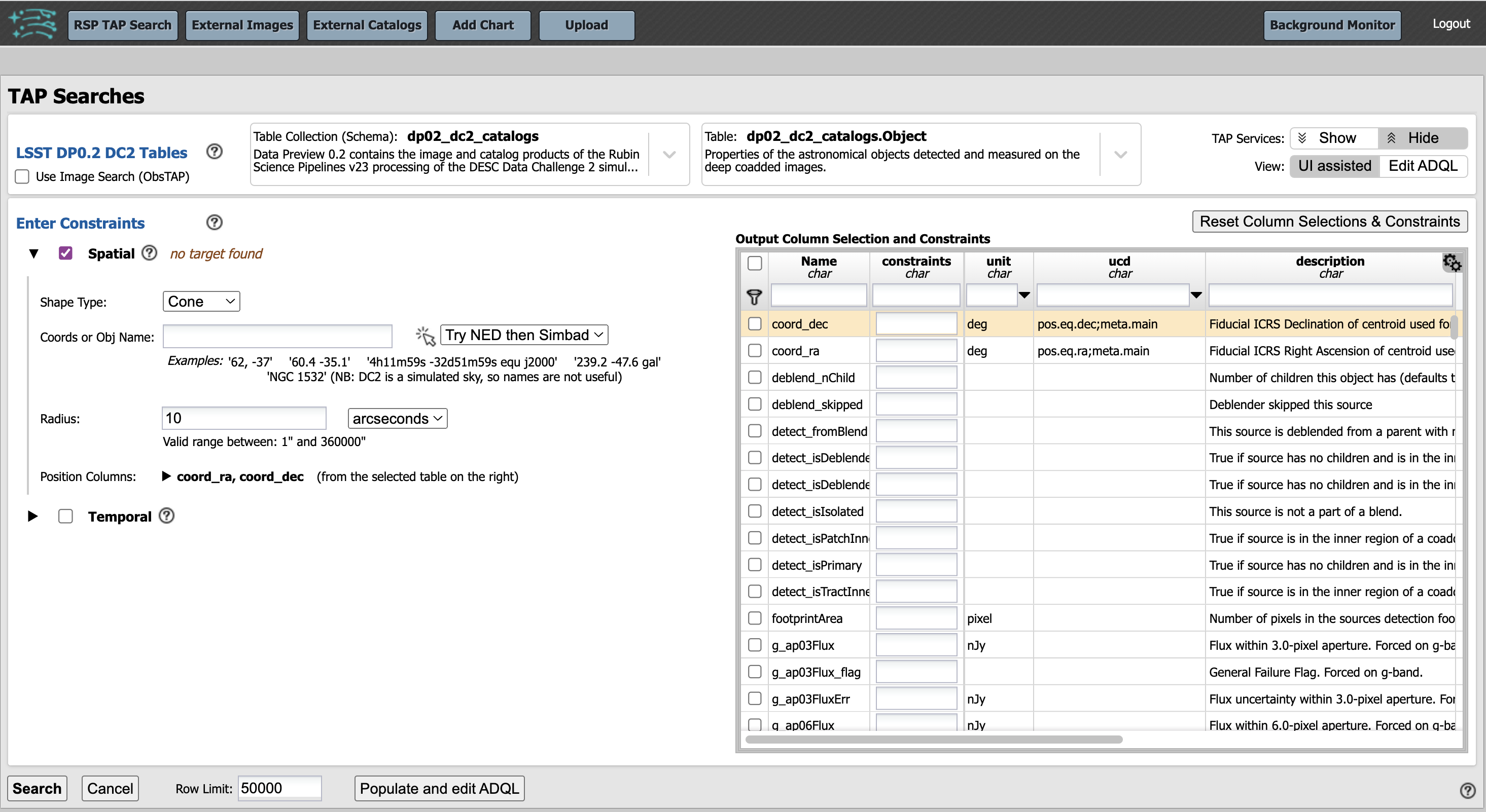
The default view of the Portal Aspect.

1.2. To access the DP0.3 TAP Service (DP0.2 is the default), in the upper right corner next to “TAP Services” click “Show”. A new option will appear at the top, called “Select TAP Service”. Click on where it says “Using LSST DP0.2 DC2”, and select “LSST DP0.3 SSO” from the drop-down menu. In the upper right corner next to “TAP Services” click “Hide”.

1.3. The top of the page now displays “LSST DP0.3 SSO Tables”. The default “Table Collection (Schema)” will be “dp03_catalogs_10yr” and the default “Table” will be “dp03_catalogs_10yr.DiaSource”. Change the “Table” to be “dp03_catalogs_10yr.MPCORB”. Notice how the area under “Enter Constraints” automatically un-checks the “Spatial Constraints” box, as the MPCORB table does not contain sky coordinates, and how the table under “Output Column Selection and Constraints” automatically updates to display the columns of the MPCORB table.

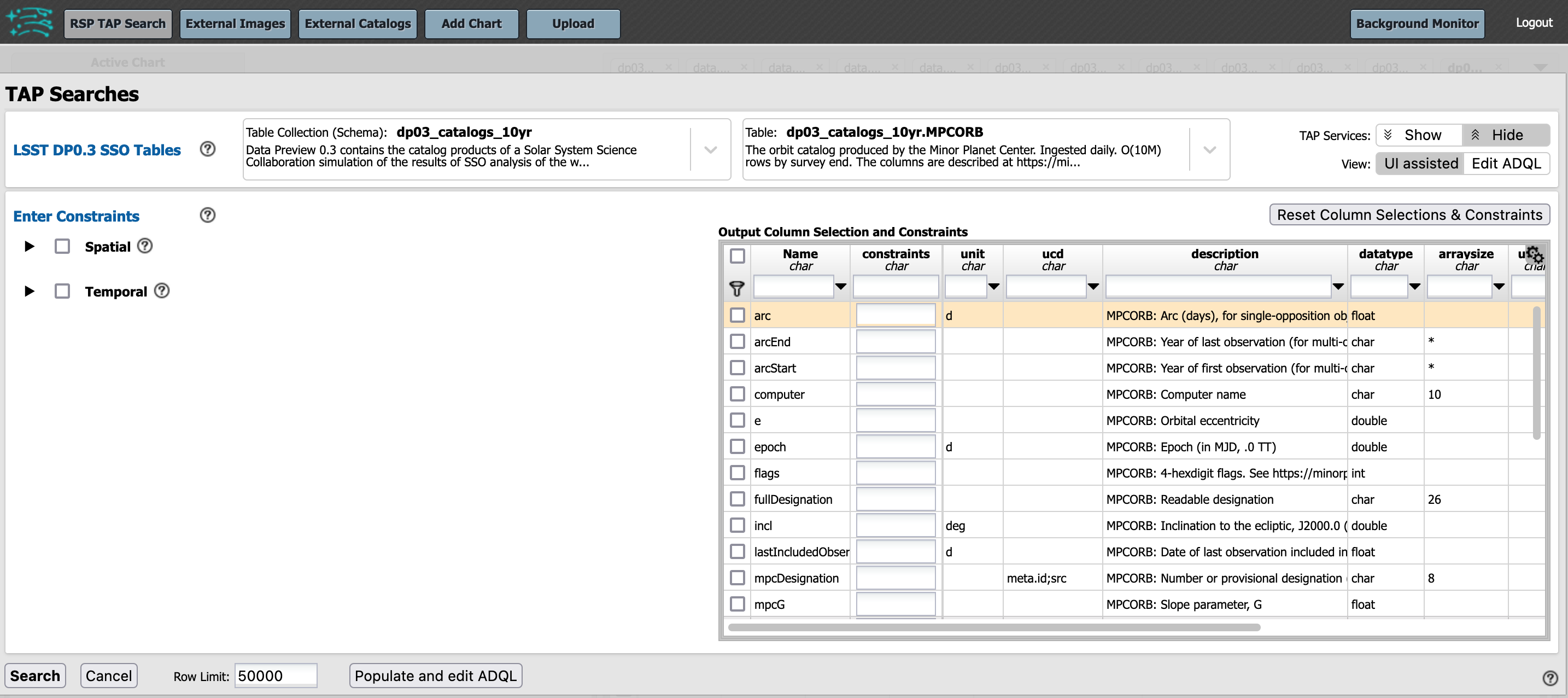
The Portal interface is prepared to query the MPCORB table.

1.4. Set up a query to retrieve the eccentricity, inclination, and absolution magnitude H for 50000 bright objects in the MPCORB table. First, click the selection box next to each column name to be returned: eccentricity (e), inclination (incl), and absolute magnitude H (mpcH). Click the funnel icon at the top of the column of selection boxes to view only selected columns. In the “constraints” box in the row for the mpcH column, enter “< 20” to return only moving objects with absolute magnitudes “H < 20” mag. At the bottom, leave the “Row Limit” set at the default of “50000”.

WARNING: The 50000 objects returned will not be a truly random sample, they will be any 50000 objects in the table that match the query conditions. Tables are typically sorted on some axis, and so this kind of query can preferentially return objects in a region of parameter space. Step 2 will demonstrate a way of obtaining a random sample of DP0.3 objects.

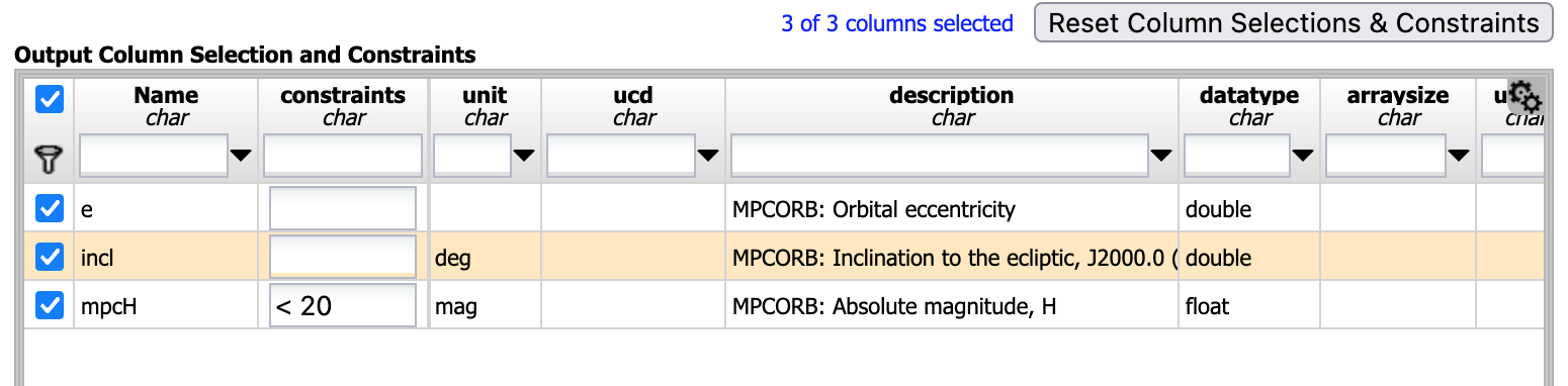
The Portal interface with the described query set up.

1.5. At lower left, click on “Search”, and the Portal will execute the query and display the default results view. The default plot is a 2-d histogram for the first two columns, eccentricity and inclination.

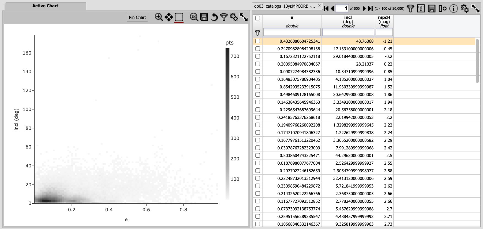
The default results view, with a plot at left and the table of results at right.

1.6. Create a histogram of the eccentricity values. In the plot panel, click on the “Settings” icon (double gears) to get the “Plot Parameters” pop-up window. Click on “Add New Chart”. Next to “Plot Type”, select “Histogram” from the drop-down menu. Next to “Column or expression” enter “e”, the column name containing the eccentricity values. Set the “Min” and “Max” values to 0 and 1, and the “Bin width” will automatically update to 0.02.

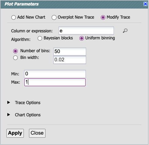
The “Plot Parameters” pop-up window set to create a histogram of eccentricities.

1.7. Click “OK” and a new plot panel containing the eccentricity histogram will appear next to the default plot panel. To get rid of the default histogram, click on the blue cross in the upper right corner of that plot to close it. Now only the eccentricity histogram appears.

1.8. Repeat steps 1.6 and 1.7 to add new plots containing the histograms for inclination and absolute magnitude. Shrink the table horizontally by clicking on the left-hand edge of the table and sliding it over to the right, making more room for the three plots.

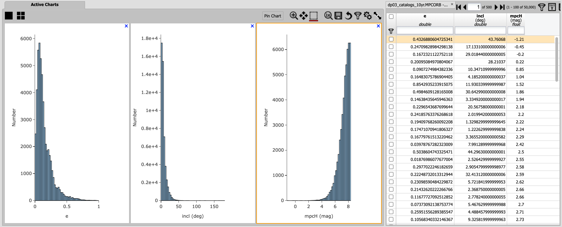
The adjusted Portal results viewer, with three histograms and a narrow table.

1.9. With the absolute magnitude plot selected (it will have an orange boundary), click on the “Settings” icon and adjust the “Plot Parameters”. Change the number of bins to 30. Under “Trace Options”, next to “Color”, click on the magnifying glass to select a new hue from the Color Picker pop-up window. Under “Chart Options”, set the title to “H Histogram” and select box to log the y-axis.

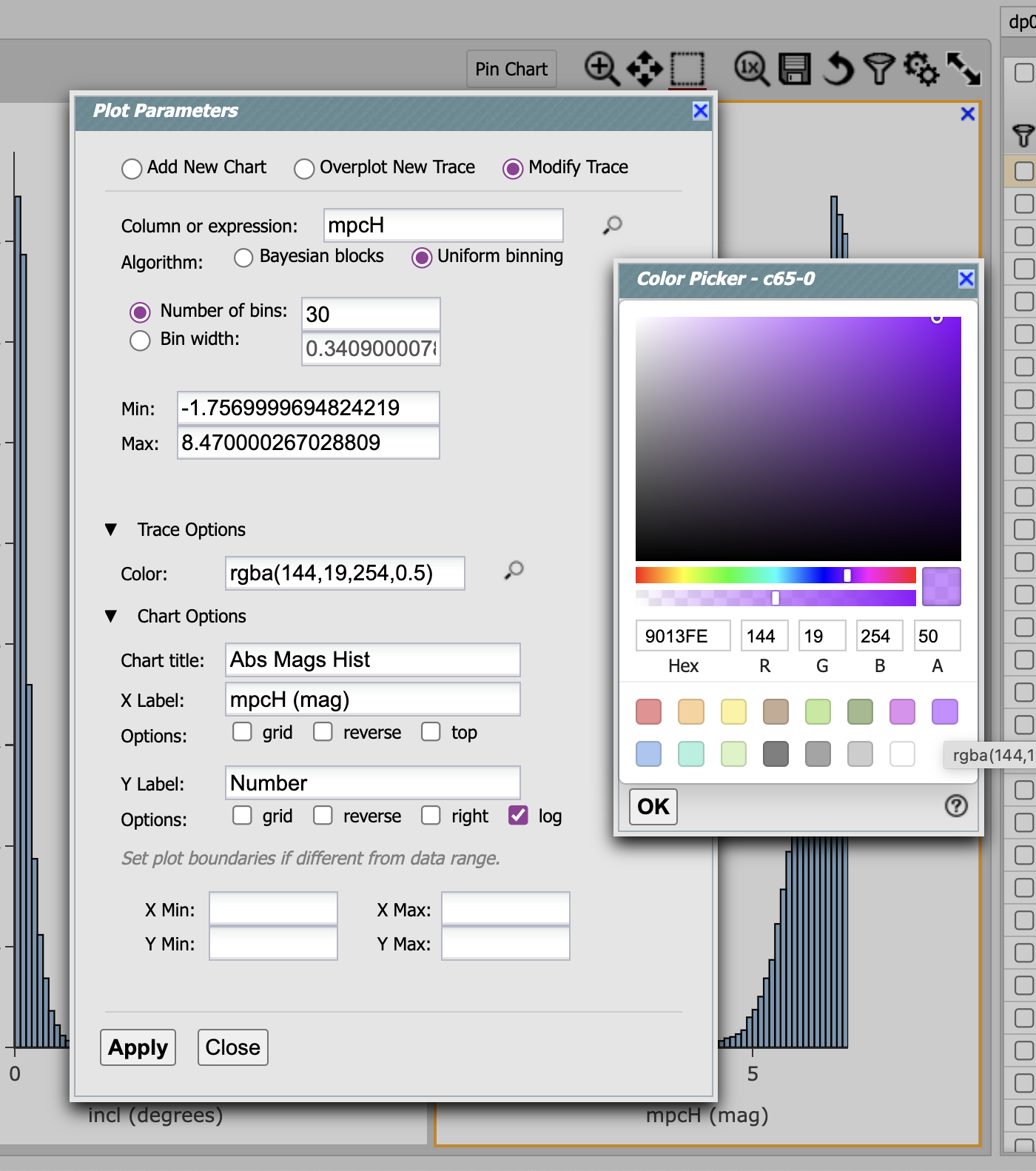
Use the “Plot Parameters” and “Color Picker” pop-up windows to adjust the appearance.

1.10. Click “Apply”, and close the pop-up windows. The absolute magnitude histogram will have the changes applied. Follow step 1.9 to adjust the appearance of the other two histograms.

1.11. To delete these search results and return to the query interface, click on the ‘x’ in the tab in the table, next to where it says “dp03_catalogs_10yr.MPCORB”. The Portal will return to the query interface. Click on “Reset Column Selections & Constraints” above the table interface to remove the previous query. Refreshing the browser window is another way to return the Portal to its default, pre-query state.

Step 2. Create a color-color diagram from the SSObject table

A random sample of DP0.3 SSObjects: As mentioned under step 1.4 above, subsets returned by applying a row limit to Portal queries are not random. To retrieve a random subset, make use of the fact that ssObjectId is a randomly assigned 64-bit long unsigned integer. Since ADQL interprets a 64-bit long unsigned integer as a 63-bit signed integer, these range from a very large negative integer value to a very large positive integer value. This will be fixed in the future so that all identifiers are positive numbers.

2.1. Follow steps 1.1 and 1.2 above, and then at upper right, next to “View” click on “Edit ADQL”. Enter the following ADQL statement into the “ADQL Query” box in order to return a count of the number of rows and the minimum and maximum values of the ssObjectId. Click “Search” in the lower left corner.

SELECT COUNT(ssObjectId), MIN(ssObjectId), MAX(ssObjectId)
FROM dp03_catalogs_10yr.SSObject

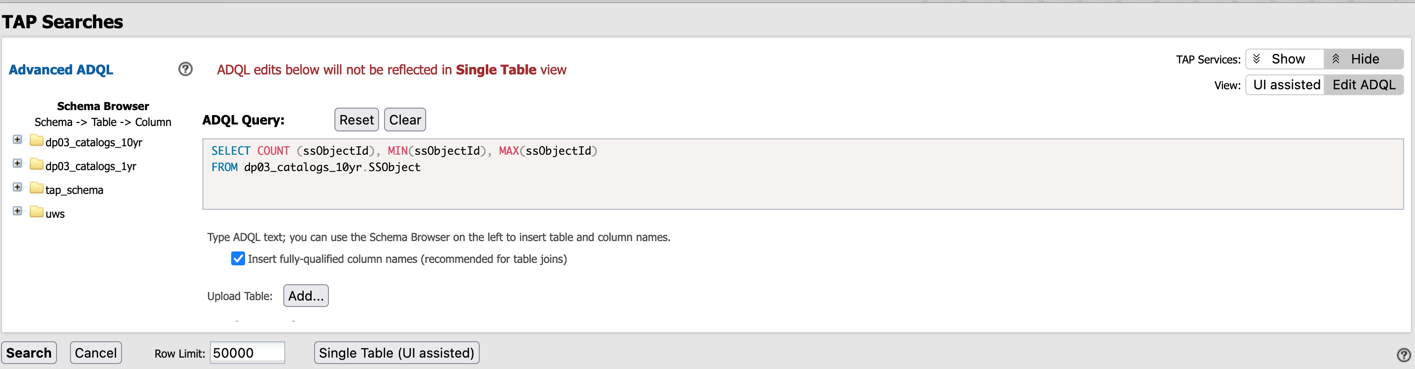
Note that there has to be a space after MAX(ssObjectId).

2.2. The results view will look similar that in step 1.5 above, but for this query the default plot is not helpful. Obtaining the values in the table were the only objective of this first query.

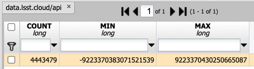
The results view table of the counts, minimum, and maximum values of ssObjectId.

2.3. Notice that the SSObject table contains roughly 4.4 million moving objects. Comparing this to the size of the MPCORB table is left as an exercise for the learner, below.

2.4. As the maximum value of the ssObjectId is 9223370430250665087, a random subset of SSObjects that contains no more than 3% of the total number (about 120,000) can be returned by applying a constraint that ssObjectId must be greater than 8660000000000000000 (i.e., because \(922 - 0.06 \times 922 \approx 866\)).

2.5. As in step 1.11 above, delete the results of this query and return to the Portal’s search interface. Clear the past query from the ADQL box.

2.6. Enter the following query to retrieve the g, r, i, and z absolute H magnitudes for a random subset of the SSObject table. Before clicking “Search”, increase the row limit to 200000.

SELECT g_H, r_H, i_H, z_H
FROM dp03_catalogs_10yr.SSObject
WHERE ssObjectId > 8660000000000000000

2.7. The default results view displays a plot of the r- vs. the g-band absolute H magnitude at left. At right, the table shows that absolute H magnitudes were not derived for all objects.

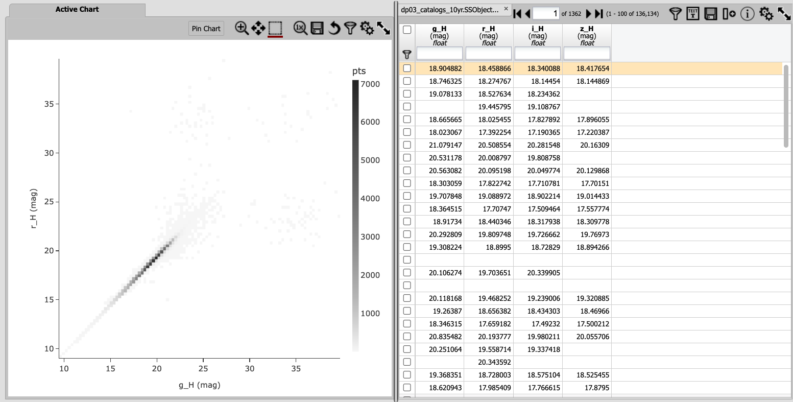
The default results view for the retrived subset of 136,134 random SSObjects.

2.8. In the plot panel, click on the “Settings” icon at upper right (the double gears) and in the “Plot Parameters” pop-up window, “Modify Trace” to have “X” be g_H - r_H and “Y” be i_H - z_H. Set the “Color Scale” to Earth. Set the “Number of X-Bins” and “Number of Y-Bins” to be 200. Under “Chart Options”, set the “X Label”, “Y Label”, “X Min”, “X Max”, “Y Min”, and “Y Max” values as in the screenshot below.

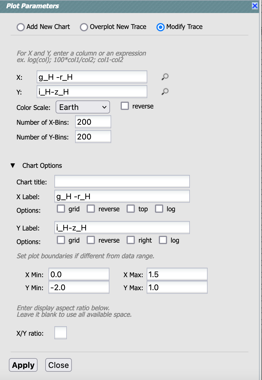
Adjust the “Plot Parameters” to create a color-color diagram.

2.9. Click “Apply” and view the color-color diagram.

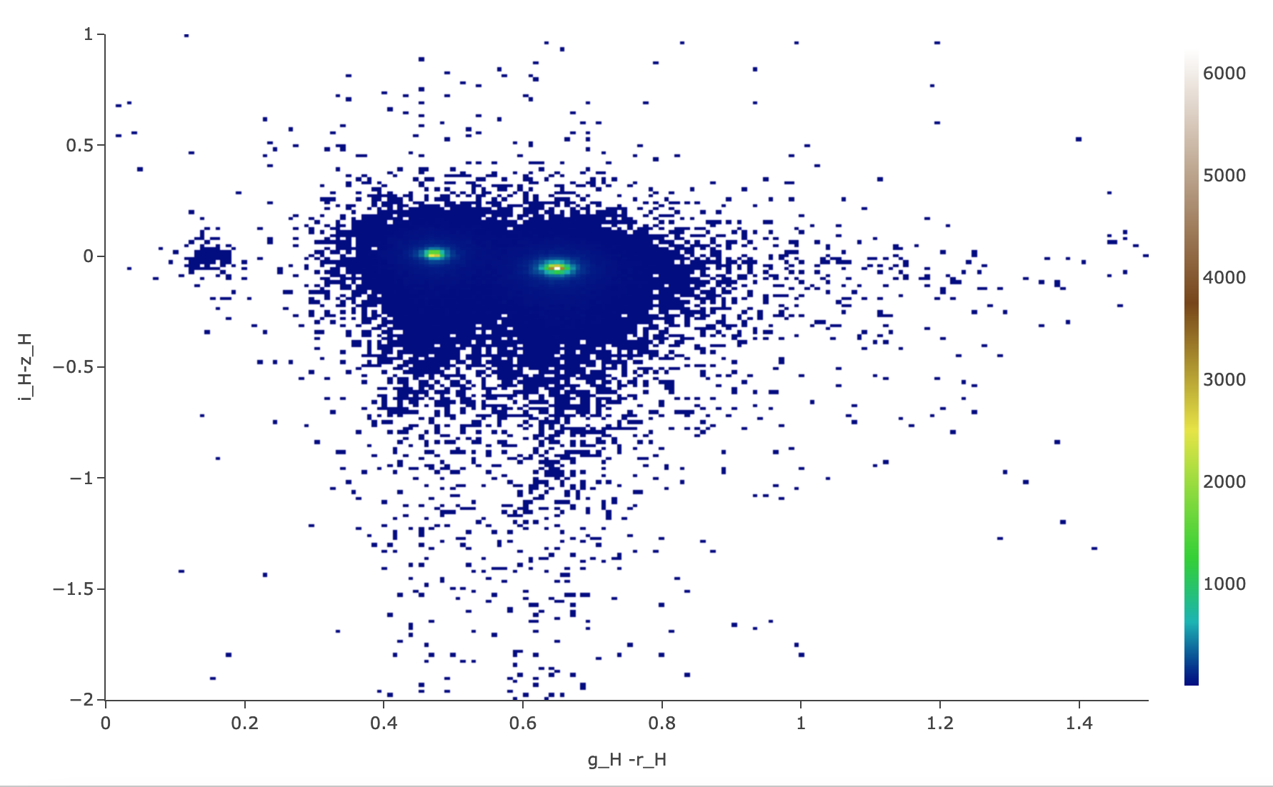
The color-color diagram for a random subset of SSObjects.

2.10. View the plot, and notice that there are two populations of colors in the simulation. This is not the case for real Solar System objects. These plots will look very different in the future, when they are made with real Rubin data. Adjusting the plot parameters is left as an exercise for the learner.

Step 3. Exercises for the learner

3.1. How big is the MPCORB table? It is larger than the SSObject table because the MPC contains all of the moving objects ever reported by anyone, based on observations from any survey, whereas the SSObject table contains only moving objects detected by LSST. Which populations of moving objects does LSST not detect?

3.2. Explore and adjust the color-color plot. To zoom in, click on the the magnifying glass with the + symbol above the plot panel, then click-and-drag in the plot. Reopen the plot parameter pop-up window and use 500 bins instead of 200. Try different color scales. Try plotting different color combinations or create a color-magnitude diagram.