01. Introduction to DP0.3: the MPCORB and SSObject catalogs (beginner)

RSP Aspect: Portal

Contact authors: Greg Madejski and Melissa Graham

Last verified to run: February 13, 2025

Targeted learning level: Beginner

Credits: This tutorial incorporates material from the introductory DP0.3 tutorial notebook by Douglas Tucker and Bob Abel.

Introduction

This tutorial demonstrates how to access the simulated Data Preview 0.3 (DP0.3) data set in the Rubin Science Platform’s Portal Aspect.

For the DP0.3 simulation, only moving objects were simulated, and only catalogs were created (there are no images). The DP0.3 simulation is entirely independent of and separate from the DP0.2 simulation. DP0.3 is a hybrid catalog that contains both real and simulated Solar System objects (asteroids, near-Earth objects, Trojans, trans-Neptunian objects, comets, and even a few spaceships… but no major planets). See The Simulated Data Set for more information about how the hybrid catalog was created.

For DP0.3 there are two catalogs, one is representative of the Solar System data products after one year of the LSST, and the other after 10 years (dp03_catalogs_1yr and dp03_catalogs_10yr, respectively). This tutorial uses the 10-year simulation.

Both DP0.3 catalogs contain four tables: MPCORB, SSObject, SSSource, and DiaSource. Their contents are described in the DP0.3 Data Products Definition Document (DPDD). In Rubin Operations, these tables would be constantly changing, updated every day with the results of the previous night’s observations. However, for DP0.3, static catalogs have been simulated.

This tutorial focuses on the first two tables, MPCORB and SSObject and it will explore these tables individually. The table joins will be demonstrated in DP0.3 Portal Tutorial 02. That tutorial will focus on SSSource and DiaSource tables. It will also illustrate, among other things, how to extract and plot the magnitude, the heliocentric, and the topocentric position of an object vs. time.

For more information about Rubin’s plans for Solar System Processing, see The Solar System Processing (SSP) Pipeline page.

TAP and ADQL

The DP0.3 data sets are available via the Table Access Protocol (TAP) service via the Portal Aspect, and can be queried via either the “UI Assisted” table interface, or via the ADQL (Astronomical Data Query Language) interface. This tutorial will demonstrate both interfaces. TAP provides standardized access to catalog data for discovery, search, and retrieval. Full documentation for TAP is provided by the International Virtual Observatory Alliance (IVOA). ADQL is similar to SQL (Structured Query Language). The documentation for ADQL includes more information about syntax and keywords.

Step 1. Plot histograms of orbital elements in the MPCORB table

1.1. Log in to the Rubin Science Platform at data.lsst.cloud and select the Portal Aspect.

1.2. Since you will be working with the DP0.3 data, select the “DP0.3 Catalogs” tab on top of the page. This will bring you to the default landing page of Portal’s DP0.3 page.

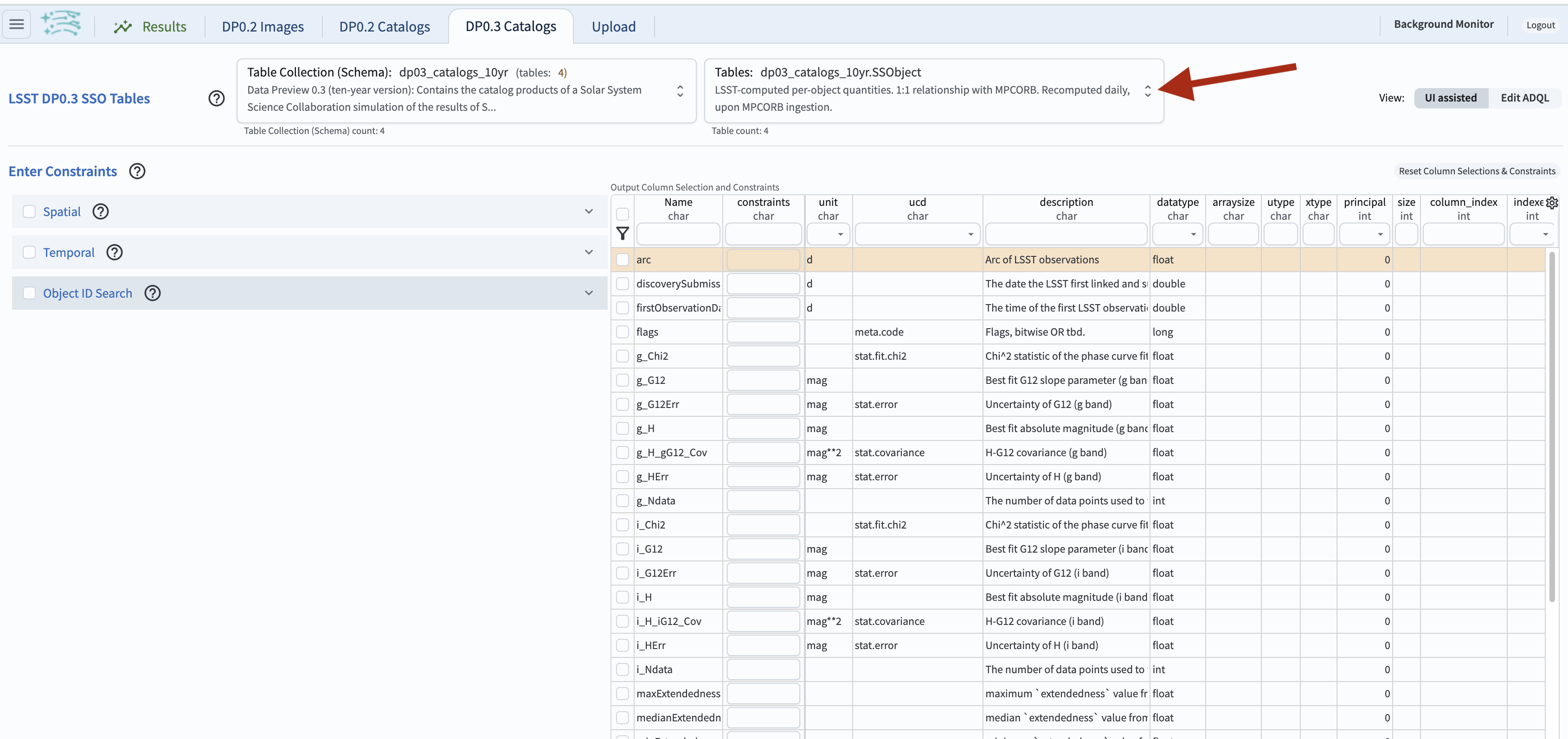
Figure 1: The default view of the Portal Aspect after selecting the “DP0.3 Catalogs” tab in the RSP Portal aspect.

1.3. The top left part of the page now displays “LSST DP0.3 SSO Tables”. The default “Table Collection (Schema)” will be “dp03_catalogs_10yr” and the default “Table” will be “dp03_catalogs_10yr.SSObject”. Click the double-arrow in the “Tables” tab and change the table to be “dp03_catalogs_10yr.MPCORB”. Notice how the table under “Output Column Selection and Constraints” automatically updates to display the columns of the MPCORB table.

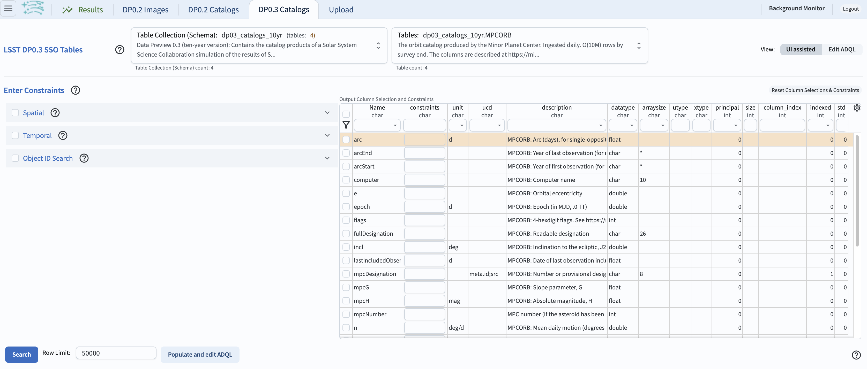
Figure 2: The Portal interface, prepared to query the MPCORB table.

1.4. Set up a query to retrieve the eccentricity, inclination, and absolute magnitude H for 50000 bright objects in the MPCORB table. First, click the selection box next to each column name to be returned: eccentricity (e), inclination (incl), and absolute magnitude H (mpcH). Click the funnel icon at the top of the column of selection boxes to view only selected columns. In the “constraints” box in the row for the mpcH column, enter “< 20” to return only moving objects with absolute magnitudes “H < 20” mag. At the bottom, leave the “Row Limit” set at the default of “50000”.

WARNING: The 50000 objects returned will not be a truly random sample, they will be any 50000 objects in the table that match the query conditions. Tables are typically sorted on some axis, and so this kind of query can preferentially return objects in a region of parameter space. Step 2 will demonstrate a way of obtaining a random sample of DP0.3 objects.

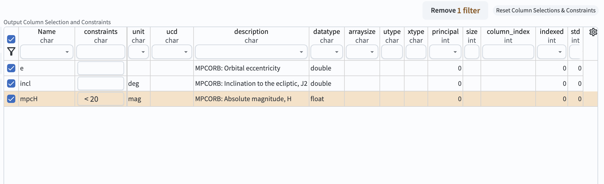
Figure 3: The Portal interface with the described query set up.

1.5. At lower left, click on “Search”, and the Portal will execute the query and display the default results view. The default plot is a 2-d histogram for the first two columns, eccentricity and inclination.

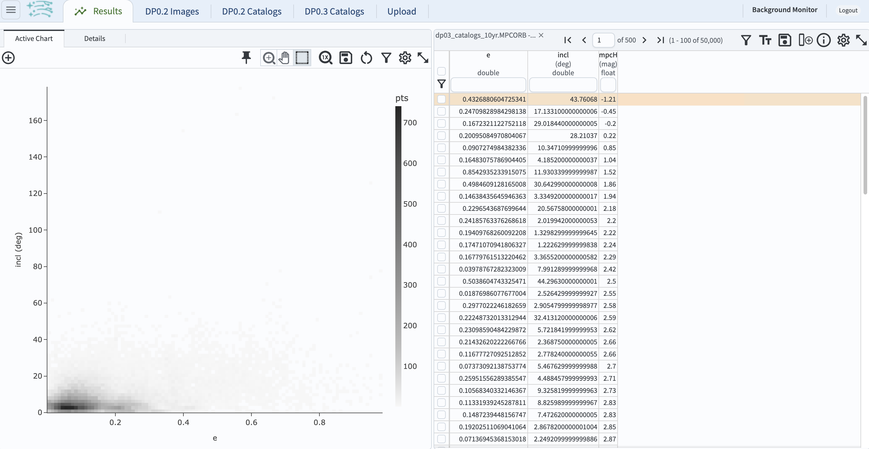
Figure 4: The default results view, with a plot at left and the table of results at right.

1.6. Create a histogram of the eccentricity values. Add a new chart by clicking on the “+” sign on the upper left. This will bring up a new “Add new chart” pop-up window. Next to “Plot Type”, select “Histogram” from the drop-down menu. Next to “Column or expression” enter “e”, the column name containing the eccentricity values. Set the “Min” and “Max” values to 0 and 1, and select the “Bin width”, which will automatically update to 0.02.

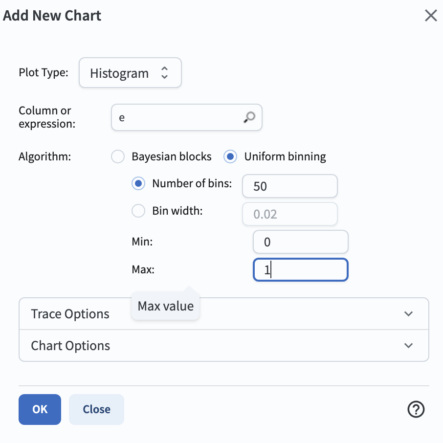
Figure 5: The “Plot Parameters” pop-up window set to create a histogram of eccentricities.

1.7. Click “OK” and a new plot panel containing the eccentricity histogram will appear next to the default plot panel. To get rid of the default histogram, click on the black cross in the upper right corner of that plot to close it. Now only the eccentricity histogram appears.

1.8. Repeat steps 1.6 and 1.7 to add new plots containing the histograms for inclination and absolute magnitude, using the default “Min”, “Max”, and “Bin Width” values. Shrink the table horizontally by clicking on the left-hand edge of the table and sliding it over to the right, making more room for the three plots.

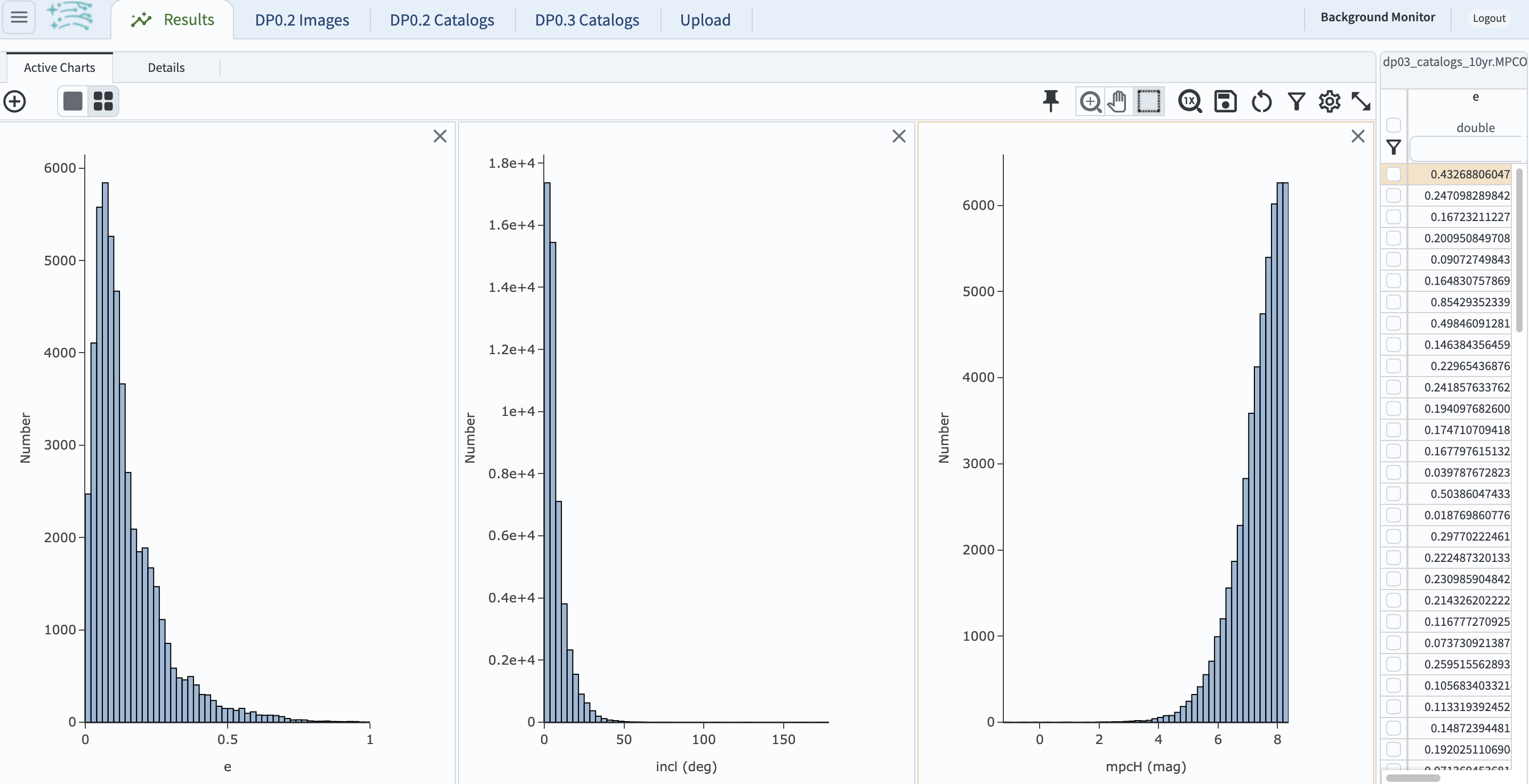
Figure 6: The adjusted Portal results viewer, with three histograms and a narrow table.

1.9. With the absolute magnitude plot selected (it will have an orange boundary), click on the “Settings” icon and adjust the “Plot Parameters”. Change the number of bins to 30. Under “Trace Options”, next to “Color”, click on the magnifying glass to select a new hue from the Color Picker pop-up window. Under “Chart Options”, set the title to “H Histogram” and select the box to log the y-axis.

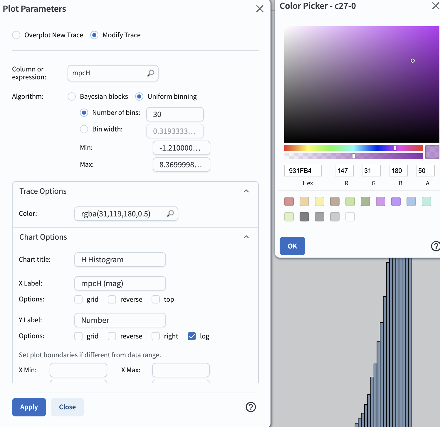
Figure 7: The use of the “Plot Parameters” and “Color Picker” pop-up windows to adjust the appearance.

1.10. Click “Apply”, and close the pop-up windows. The absolute magnitude histogram will have the changes applied. Follow step 1.9 to adjust the appearance of the other two histograms.

1.11. To delete these search results and return to the query interface, click on the ‘x’ in the tab in the table, next to where it says “dp03_catalogs_10yr.MPCORB”. The Portal will return to the interface where you select the catalog set. Select the “DP0.3 Catalogs” tab once again. Click on “Reset Column Selections & Constraints” above the table interface to remove the previous query. Refreshing the browser window is another way to return the Portal to the state corresponding to the first time you clicked on “DP0.3 Catalogs” tab upon logging into the RSP.

Step 2. Create a color-color diagram from the SSObject table

A random sample of DP0.3 SSObjects: As mentioned under step 1.4 above, subsets returned by applying a row limit to Portal queries are not random. To retrieve a random subset, make use of the fact that ssObjectId is a randomly assigned 64-bit long unsigned integer. Since ADQL interprets a 64-bit long unsigned integer as a 63-bit signed integer, these range from a very large negative integer value to a very large positive integer value. This will be fixed in the future so that all identifiers are positive numbers.

2.1. Follow steps 1.1 and 1.2 above, and then at upper right, next to “View” click on “Edit ADQL”. Enter the following ADQL statement into the “ADQL Query” box in order to return a count of the number of rows and the minimum and maximum values of the ssObjectId. Click “Search” in the lower left corner.

SELECT COUNT(ssObjectId), MIN(ssObjectId), MAX(ssObjectId)
FROM dp03_catalogs_10yr.SSObject

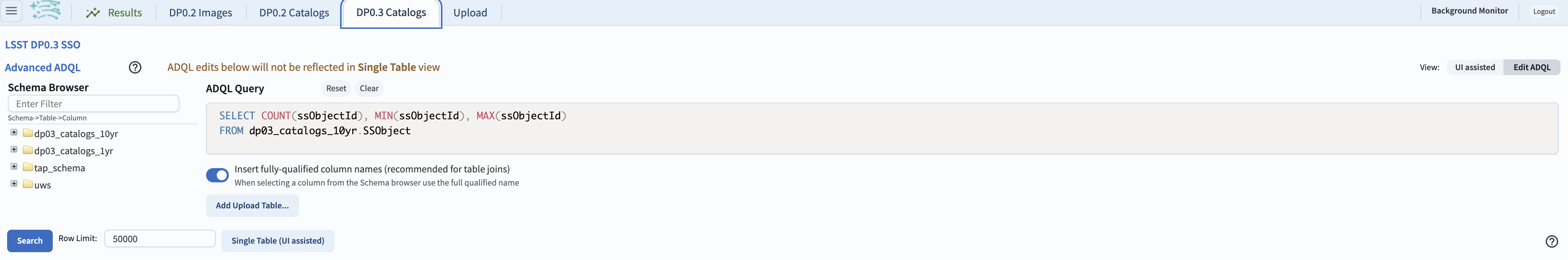
Figure 8: A screenshot of the ADQL entry to select the number of observations, and the range of ssObjectId values on the SSObject table.

2.2. The results view will look similar to that in step 1.5 above, but for this query the default plot is not helpful. Obtaining the values in the table was the only objective of this first query.

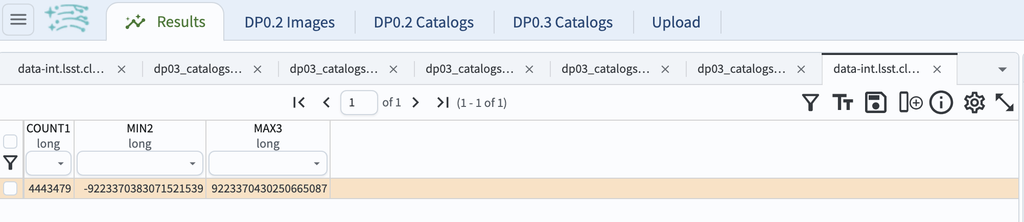
Figure 9: The results view table of the object count, as well as the minimum and the maximum values of ssObjectId.

2.3. Notice that the SSObject table contains roughly 4.4 million moving objects. Comparing this to the size of the MPCORB table is left as an exercise for the learner, below.

2.4. As the maximum value of the ssObjectId is 9223370430250665087, a random subset of SSObjects that contains no more than 6% of the total number (about 120,000) can be returned by applying a constraint that ssObjectId must be greater than 8660000000000000000 (i.e., because \(922 - 0.06 \times 922 \approx 866\)).

2.5. As in step 1.11 above, delete the results of this query and return to the Portal’s search interface. Clear the past query from the ADQL box.

2.6. Enter the following query to retrieve the g, r, i, and z absolute H magnitudes for a random subset of the SSObject table. Before clicking “Search”, increase the row limit to 200000.

SELECT g_H, r_H, i_H, z_H
FROM dp03_catalogs_10yr.SSObject
WHERE ssObjectId > 8660000000000000000

2.7. The resulting view displays a plot of the r- vs. the g-band absolute H magnitude at left. At left, the table shows that absolute H magnitudes were not derived for all objects.

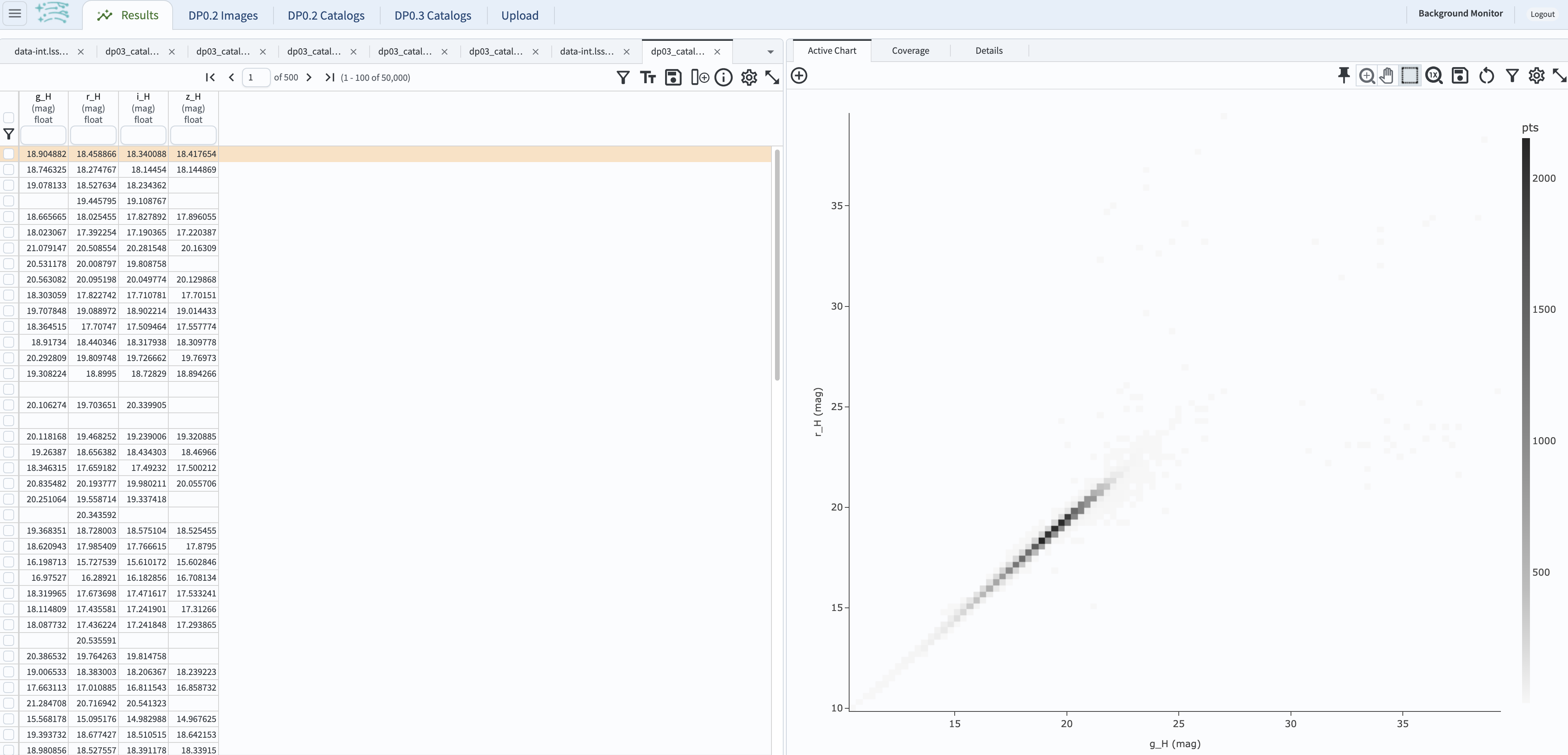
Figure 10: The default results view for the retrieved subset of 136,134 random SSObjects.

2.8. In the plot panel, click on the “Settings” icon at upper right (the single gear) and in the “Plot Parameters” pop-up window, “Modify Trace” to have “X” be g_H - r_H and “Y” be i_H - z_H. Set the “Color Scale” to “YlGnBu”. Set the “Number of X-Bins” and “Number of Y-Bins” to be 200. Note that the maximum number of bins in such “heatmap” plots in both X and Y is 300. Under “Chart Options”, set the “X Label”, “Y Label”, “X Min”, “X Max”, “Y Min”, and “Y Max” values as in the screenshot below.

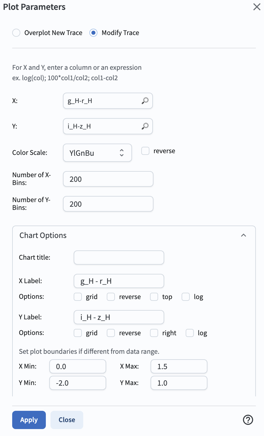
Figure 11: Pop-up window with the “Plot Parameters” to create a color-color diagram.

2.9. Click “Apply” and view the color-color diagram.

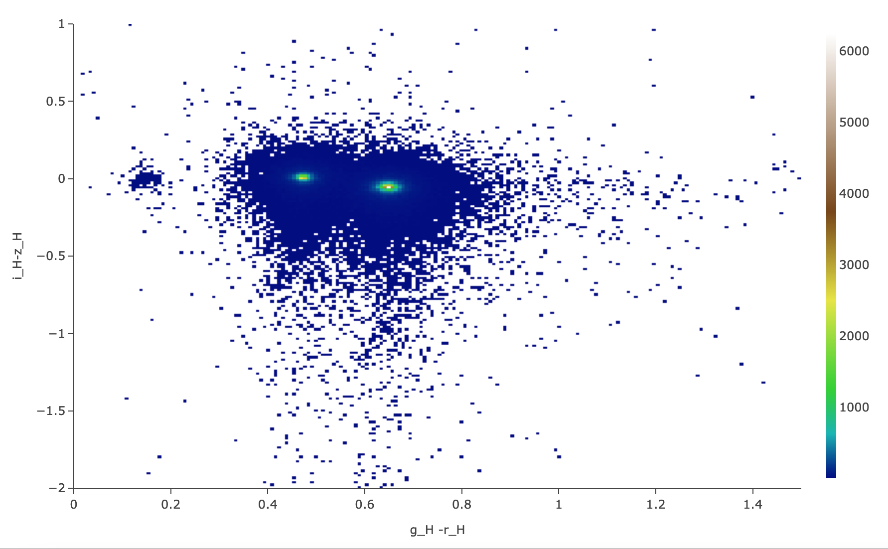
Figure 12: The color-color diagram for a random subset of SSObjects.

2.10. View the plot, and notice that there are two sets of object colors in the simulation. This is not the case for real Solar System objects. These plots will look very different in the future, when they are made with real Rubin data. Adjusting the plot parameters is left as an exercise for the learner.

Step 3. Exercises for the learner

3.1. How big is the MPCORB table? It is larger than the SSObject table because the MPC contains all of the moving objects ever reported by anyone, based on observations from any survey, whereas the SSObject table contains only moving objects detected by LSST. Which populations of moving objects does LSST not detect?

3.2. Explore and adjust the color-color plot. To zoom in, click on the magnifying glass with the + symbol above the plot panel, then click-and-drag in the plot. Reopen the plot parameter pop-up window and use 300 bins instead of 200. Try different color scales. Try plotting different color combinations or create a color-magnitude diagram.