02. Introduction to DP0.3: the SSSource and DiaSource tables (beginner)#
RSP Aspect: Portal
Contact authors: Melissa Graham and Greg Madejski
Last verified to run: February 13, 2025
Targeted learning level: beginner
Credits: This tutorial incorporates material from the introductory DP0.3 tutorial notebook by Douglas Tucker and Bob Abel.
Introduction#
This tutorial is a direct sequel to Portal tutorial 01: Introduction to DP0.3: the MPCORB and SSObject tables.
Those two tables contain derived parameters for individual simulated Solar System objects.
This tutorial focuses on the DP0.3 SSSource and DiaSource tables, which contain measured and derived
values for individial simulated Solar System objects on a per-observation basis. Their contents are described in the DP0.3 Data Products Definition Document (DPDD). Note that there are two separate DP0.3 catalogs, dp03_catalogs_1yr and dp03_catalogs_10yr, respectively. This tutorial uses the tables in the catalog resulting from the 10-year simulation.
For more information about Rubin’s plans for Solar System Processing and how these tables will be created, see The Solar System Processing (SSP) Pipeline page.
TAP and ADQL#
The DP0.3 data sets are available via the Table Access Protocol (TAP) service via the Portal Aspect, and can be queried via either the “UI Assisted” table interface, or via the ADQL (Astronomical Data Query Language) interface. This tutorial assumes completion of Portal Tutorial 01 and only demonstrates the ADQL interface. It also llustrates how to perform table joins. ADQL is similar to SQL (Structured Query Langage). The documentation for ADQL includes more information about syntax and keywords.
Step 1. Identify an object to explore#
1.1. Log in to the Rubin Science Platform at data.lsst.cloud and select the Portal Aspect.
1.2. To access the DP0.3 TAP Service, click on the “DP0.3 Catalogs” tab at the top of the screen. The default “Table Collection (Schema)”, which is “dp03_catalogs_10yr”, will be used for this tutorial. To change the “Table” from the default “dp03_catalogs_10yr.SSObject”, click on the down arrow and selecting one of the other tables, such as the “dp03_catalogs_10yr.DiaSource” table, which will be explored in this tutorial.
1.3. At upper right, click “Edit ADQL”, and enter the following query into the box.
This query retrieves a random subset of SSObjects that were observed between 100 and 300 times
over the 10-year LSST survey simulation,
are bright (g_H < 20 mag) but would never saturate with LSST (g_H > 17 mag),
are in the inner Solar System (q < 3),
and have orbits that are inclined by at least 20 degrees and eccentricities between 0.1 and 0.5. Click the “Search” button in the lower left-hand corner.
SELECT sso.numObs, sso.g_H, sso.ssObjectId, mpc.e, mpc.incl, mpc.q
FROM dp03_catalogs_10yr.ssObject AS sso
JOIN dp03_catalogs_10yr.MPCORB AS mpc ON sso.ssObjectId = mpc.ssObjectId
WHERE (sso.ssObjectId BETWEEN 7500000000000000000 AND 8500000000000000000)
AND (sso.numObs > 100) AND (sso.numObs < 300)
AND (sso.g_H > 17) AND (sso.g_H < 20)
AND (mpc.q < 3) AND (mpc.incl > 20) AND (mpc.e > 0.1) AND (mpc.e < 0.5)
1.4. The default results view will plot the g-band absolute H magnitude versus the number of observations for the 4150 objects.
1.5. In the upper-right corner of the Active Chart panel, click the settings icon (single gear) to open the plot parameters pop-up window.
Change the y-axis column to eccentricity (e), click “Apply” and then “Close”.
Click on an object of interest and the point will turn orange and it will be highlighted in the table.
Record the ssObjectID of the chosen object.
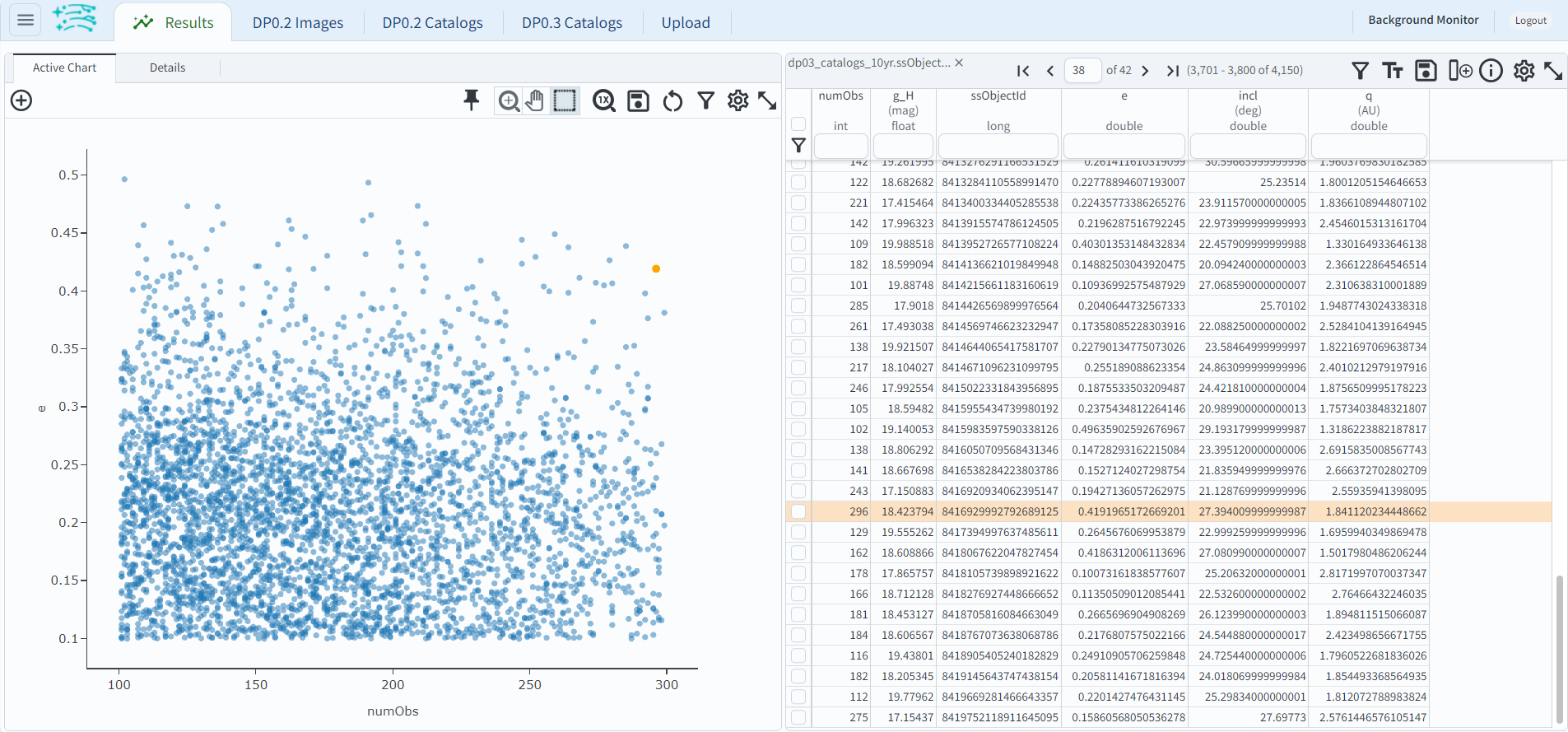
Figure 1: A screenshot of the results view, with the plot altered to show eccentricy versus number of observations.#
Step 2. Visualize the object’s orbit#
2.1. Click on “DP0.3 Catalogs” tab at the top to return to the main search page, and then “Edit ADQL”.
Submit the following query, using the ssObjectId as below (or one of your choosing).
This query returns the heliocentric (sun-centered) and topocentric (Earth-centered) 3D distances
of the object at the time of every simulated LSST observation from the SSSource table.
SELECT heliocentricX, heliocentricY, heliocentricZ,
topocentricX, topocentricY, topocentricZ, ssObjectId
FROM dp03_catalogs_10yr.SSSource
WHERE ssObjectId = 8416929992792689125
2.2. The “Results” tab at the top will display the results from the query, which plots the sun-centered orbit of heliocentricY versus heliocentricX.
Click on the plot settings icon and in the pop-up window, select “Chart Options” and then add a grid
to the x- and y-axis to more easily identify the Sun’s location at (0, 0).
Click “Apply” and “Close”.
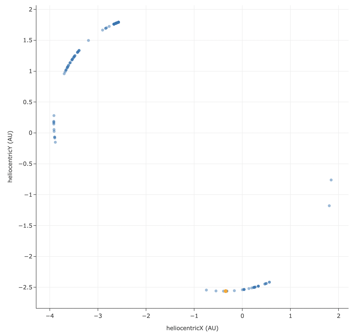
Figure 2: A visualization of the object’s orbit projected onto the plane of the Solar System.#
2.3. Add a new chart by clicking on the “+” sign on the upper left. This will bring up a new “Add new chart” pop-up window.
Create a scatter plot of the heliocentricZ (y-axis) verus heliocentricX (x-axis) with grid lines to see how this object travels out of
the plane of the Solar System due to its orbital inclination. Click “OK” and “Close”.
2.4. Add two more charts for the topocentric distances. Notice that in the topocentric distance, the object does not come near Earth (0, 0), so this is just a regular asteroid and not a hazardous one!
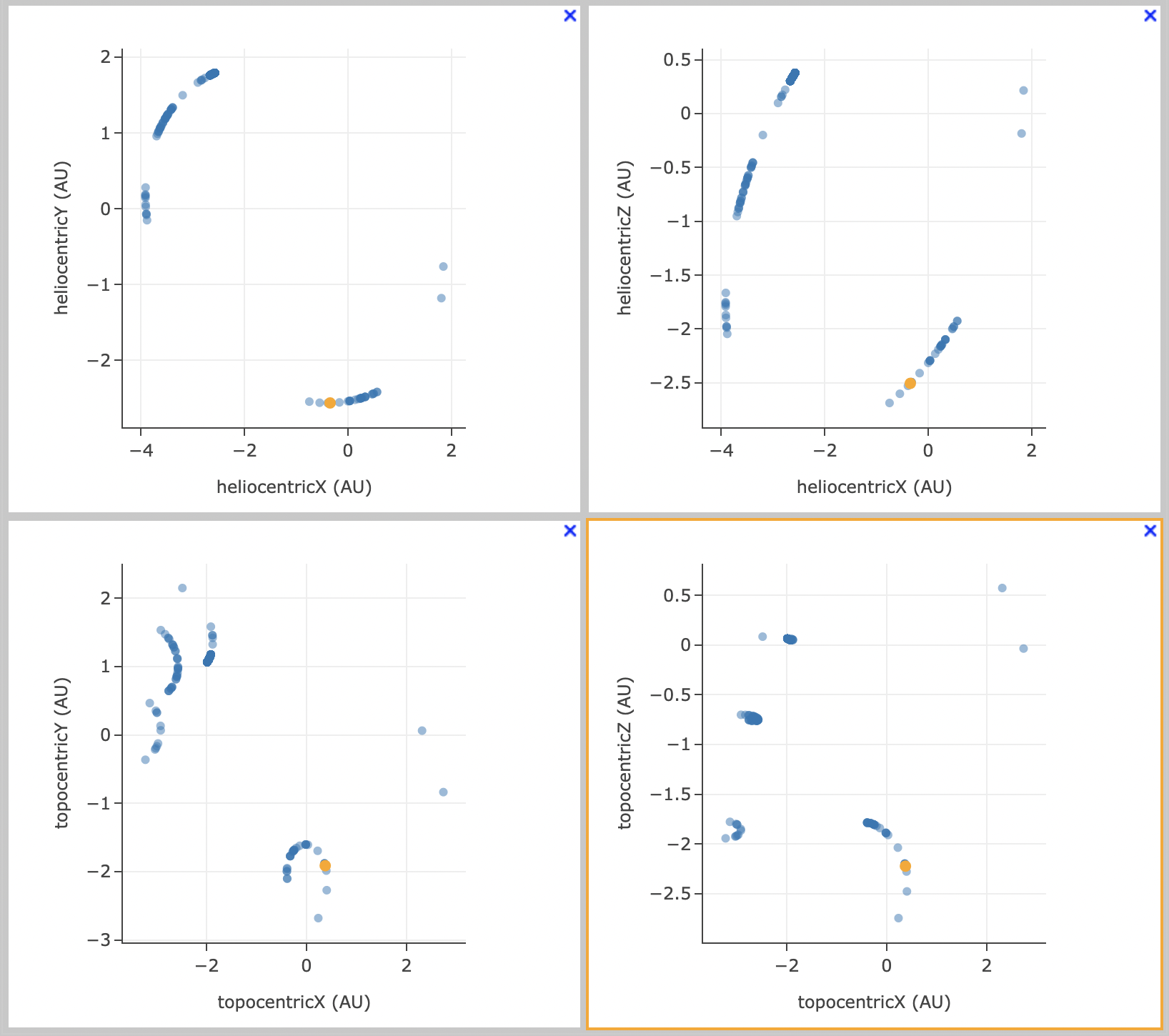
Figure 3: A visualization of the object’s orbits in heliocentric and topocentric distances.#
Step 3. Visualize the object’s 2d sky motion#
3.1. Click on “DP0.3 Catalogs” tab at the top to return to the main search page, and then “Edit ADQL”.
Submit the following query, using the same ssObjectId as above (or one of your choosing).
This query returns the right ascension (ra), declination (dec), and modified julian date
(midPointMjdTai) of every observation.
SELECT ra, dec, midPointMjdTai
FROM dp03_catalogs_10yr.DiaSource
WHERE ssObjectId = 8416929992792689125
3.2. The default results view will probably include a sky image, but since there were no images simulated for DP0.3 (catalogs only), it will be all black. Click on the “hamburger icon” (three lines in a box) at the upper left of the screen and scroll down to “Results Layout” and select “Tables and Coverage Charts” option. Click on “Active Chart” to switch between the blank “Coverage” tab and the “Active Chart Tab”.
3.3. The plot of declination versus right ascension shows how the object moves on the sky over the 10-year LSST.
Click on the settings icon (single gear) in the plot panel and in the plot parameters pop-up window,
under “Trace Options” next to “Color Map” enter midPointMjdTai, and from the drop-down menu for
“Color Scale” choose “Rainbow”.
Click “Apply” and then “Close”. This will illustrate two-dimensional motion as a function of time, which is marked as a changing color.
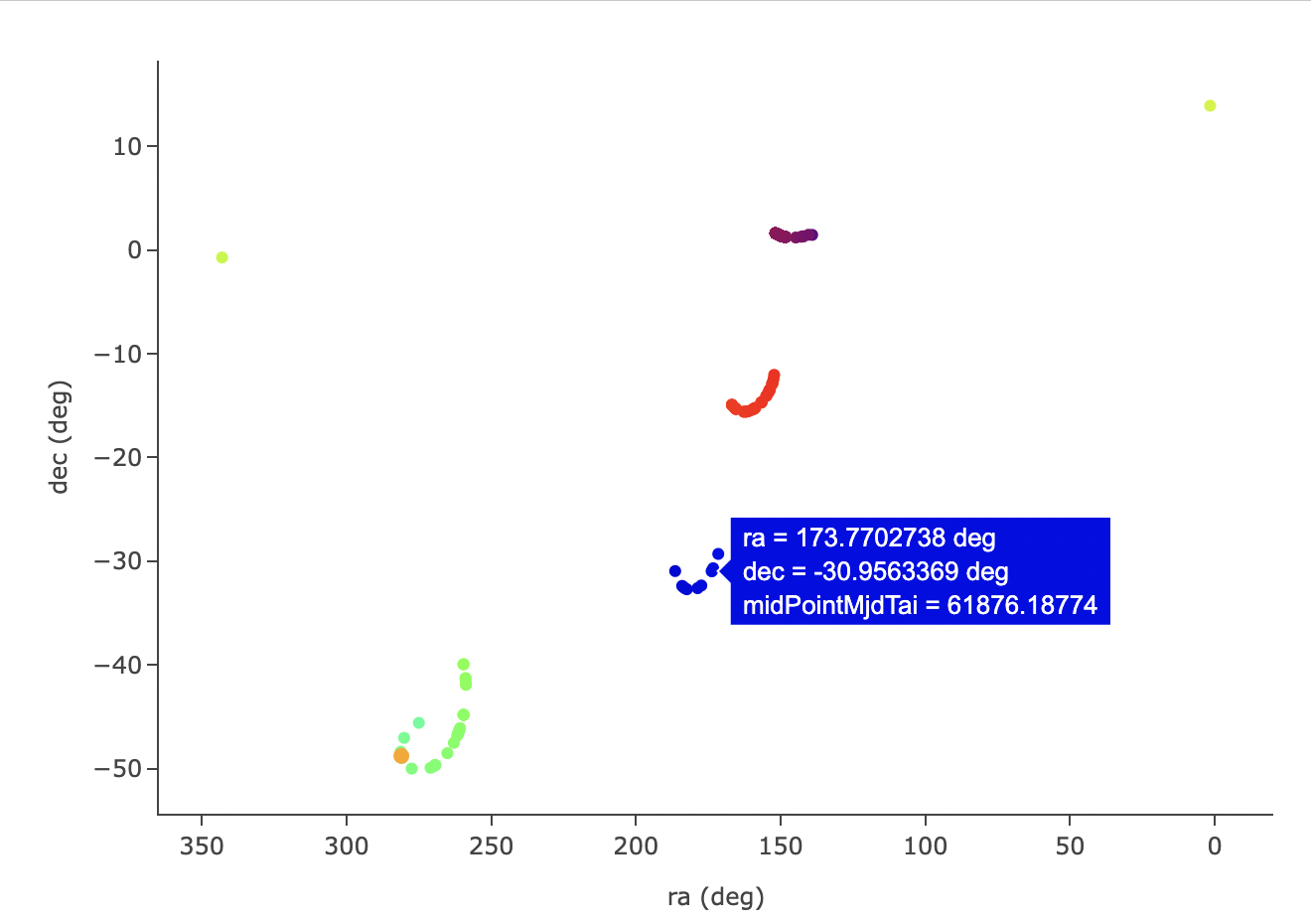
Figure 4: A visualization of the object’s motion across the sky and LSST’s detections.#
3.4. In the plot above, notice how the points are in four clusters of RA, Dec, and color. This demonstrates how the LSST observing strategy covers the moving object’s location in four years out of the ten.
Step 4. Visualize the object’s photometry#
4.1. Click on DP0.3 Catalogs to return to the search screen, and then “Edit ADQL”.
Submit the following query, using the same ssObjectId as above (or one of your choosing).
This query returns the magnitude, filter, and modified julian date (midPointMjdTai) of every
observation that was obtained in the r-band from the DiaSource table,
and the phase angle from the SSSource table.
The two tables are joined on the diaSourceId column.
SELECT dia.mag, dia.band, dia.midPointMjdTai, ss.phaseAngle
FROM dp03_catalogs_10yr.DiaSource AS dia
JOIN dp03_catalogs_10yr.SSSource AS ss ON dia.diaSourceId = ss.diaSourceId
WHERE dia.ssObjectId = 8416929992792689125
AND dia.band = 'r'
4.2. Use the plot settings icon (single gear) to open the plot parameters pop-up window, and modify the trace to
plot mag versus midPointMjdTai.
Click “Apply” and “Close”. Click the plus sign in the circle to “Add New Chart” and plot the mag as a function
of phaseAngle.
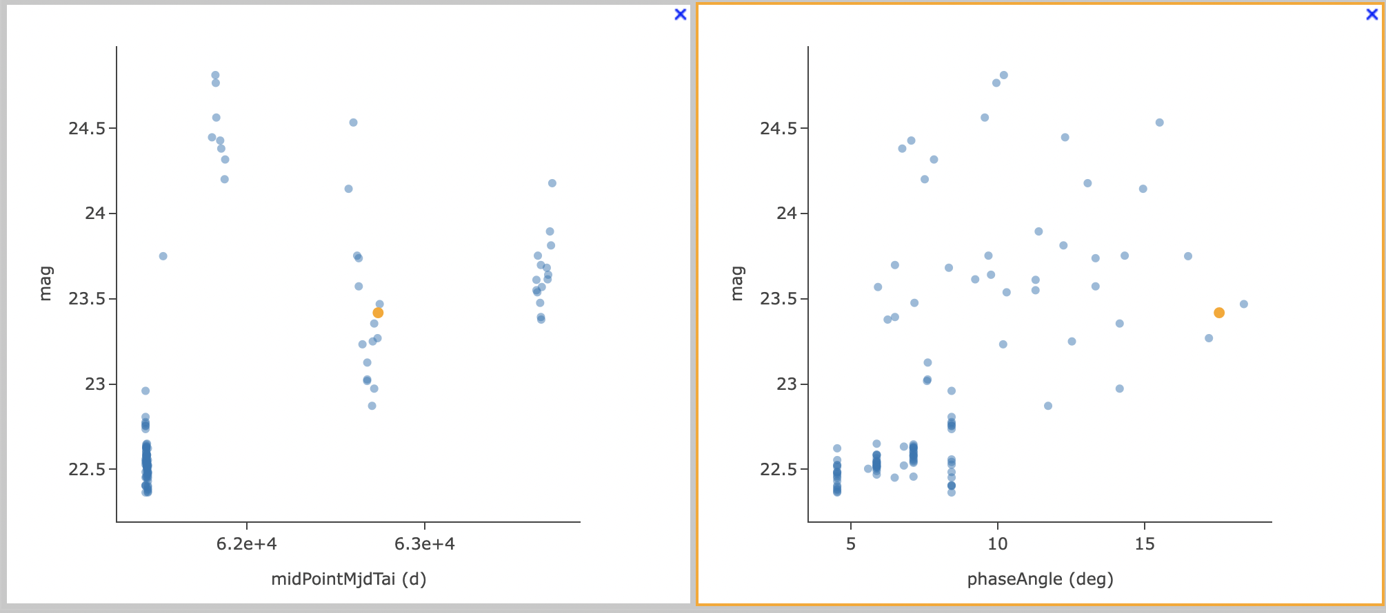
Figure 5: A visualization of the object’s magnitude changes versus time (left) and phase angle (right).#
4.3. Notice there is no trend in the magnitude as a function of time, and recall that the DP0.3 simulation does not include any time-domain changes in the photometry (e.g., rotation curves). The magnitude only depends on the distance from Earth, and the phase angle as seen from Earth. Thus, a trend emerges in the right plot, and would be clearer if the apparent magnitudes were corrected for distance. Doing this will be covered in a future tutorial.
Step 5. Exercises for the learner#
5.1. If you used ssObjectId 8416929992792689125, repeat the exercise for a different object.
5.2. The SSSource table contains instantaneous xyz velocities in addition to xyz distance.
Plot the heliocentric velocities as a function of heliocentric distance, and see the object
move slower when it is further from the Sun.
5.3. The DiaSource table contains four truth columns: raTrue, decTrue, magTrueVband,
and nameTrue.
Make a plot of the astrometric scatter in the observations (e.g., decTrue-dec versus
raTrue-ra).
5.4. Did the object with ssObjectId 8416929992792689125 have a designation or proper name in the MPC?