03. Explore Transneptunian Objects (TNOs) in DP0.3 (Intermediate)#
RSP Aspect: Portal
Contact authors: Greg Madejski and Melissa Graham
Last verified to run: March 27, 2025
Targeted learning level: Intermediate
Introduction#
This tutorial demonstrates how to identify and explore a population of transneptunian objects (TNOs) in the simulated DP0.3 catalogs.
TNOs are defined by having orbits with semimajor axes beyond the orbit of Neputne (a > 30.1 AU).
The DP0.3 simulated data set does not include the semimajor axis (a) in the MPCORB table, however it can be derived from the
orbit’s eccentricity (e) and perihelion distance (q), which are both available in the MPCORB table, via a = q/(1.0 - e).
This allows for a sample of TNOs to be identified in the DP0.3 data set (see Step 1).
TNO properties (specifically, the relationship between their semimajor axis and eccentricity, as well as the distribution of their derived diameters) will be explored in Step 2.
Note that some of the objects might have e >= 1, which means they are not bound to the Solar System and are moving on parabolic or hyperbolic orbits.
Such objects will be excluded from this tutorial, as an application of the formula above would result in a negative value of a.
Compared to the Solar System objects closer to the Earth, such as Main Belt Asteroids or Near-Earth Objects (NEOs), TNOs move relatively slowly across the sky. This relatively slow movement means that TNOs that fall within an LSST Deep Drilling Field (DDF) can stay within that field, and LSST can accumulate thousands of observations of those TNOs. This tutorial explores the position on the sky of one such TNO (Step 3) and plots time-domain quantities such as magnitude and phase angle (Step 4). Finally, it provides a visualization of its trajectory projected into 2D (see Step 5).
More information about the LSST DDFs can be found on the LSST DDF webpage and in Section 3.7 of the Survey Cadence Optimization Committee’s Phase 3 Recommendations report (PSTN-056). Note that DP0.2 did not include DDF observations, so the ability to explore science with a DDF-like cadence is unique to the DP0.3 simulation.
This tutorial assumes the successful completion of Portal tutorial 01: Introduction to DP0.3: the MPCORB and SSObject tables
and Portal tutorial 02: Introduction to DP0.3: the SSSource and DiaSource tables,
and uses the Astronomy Data Query Language (ADQL), which is similar to SQL (Structured Query Language).
For more information about the DP0.3 catalogs, tables, and columns, see the DP0.3 Data Products Definition Document (DPDD).
Step 1. Identify a population of TNOs#
1.1. Log into the Rubin Science Platform at data.lsst.cloud and select the Portal Aspect. Click on “DP0.3 Catalogs” tab to get to the “dp03_catalogs_10yr” table collection.
1.2. At upper right, next to “View” choose “Edit ADQL”.
Enter the following ADQL statement into the ADQL Query box.
It will return the eccentricity (e), perihelion distance (q), and inclination (incl) for a
random subset of objects in the MPCORB table.
For an explanation of why this constraint on ssObjectId returns a random sample, see Step 2 of
DP0.3 Portal tutorial 01: “Introduction to DP0.3: the MPCORB and SSObject tables.
SELECT e, q, incl
FROM dp03_catalogs_10yr.MPCORB
WHERE ssObjectId > 9000000000000000000
1.3. Set the “Row Limit” to be 200000 and click “Search”.
1.4. The default results view will show a heatmap plot of q vs. e at left, and the table view at right.
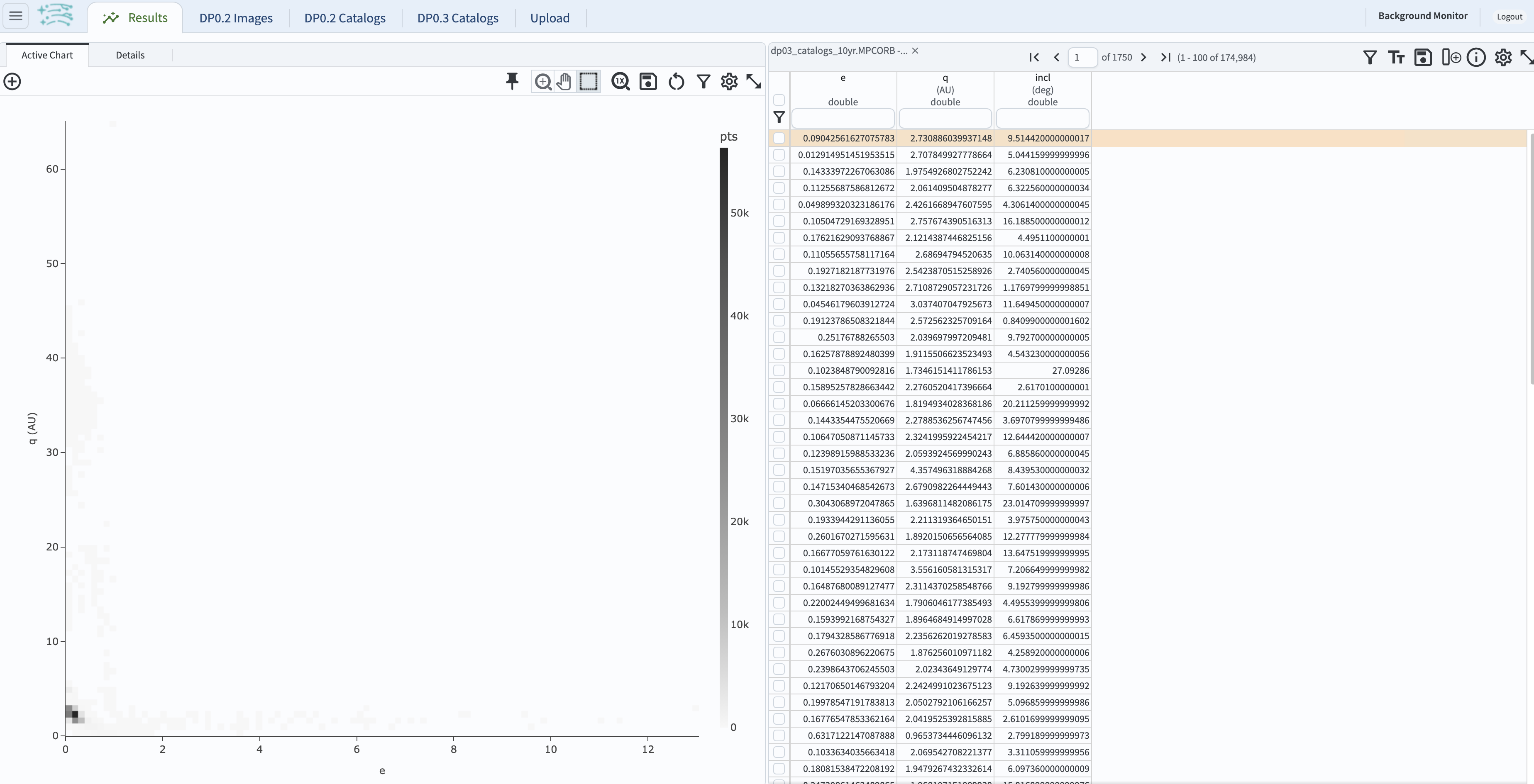
Figure 1: The default results view for the query, with the table at right and the heatmap at left.#
1.5. Exclude the objects moving on unbound orbits.
Note that a small fraction of the objects - roughly one in a thousand - have derived eccentricities > 1, which means they are not bound to the Solar System.
Those objects can be excluded from further analysis by entering < 1 in the box underneath the table heading e, and hitting “enter.”
This will result in a slightly modified display as below.
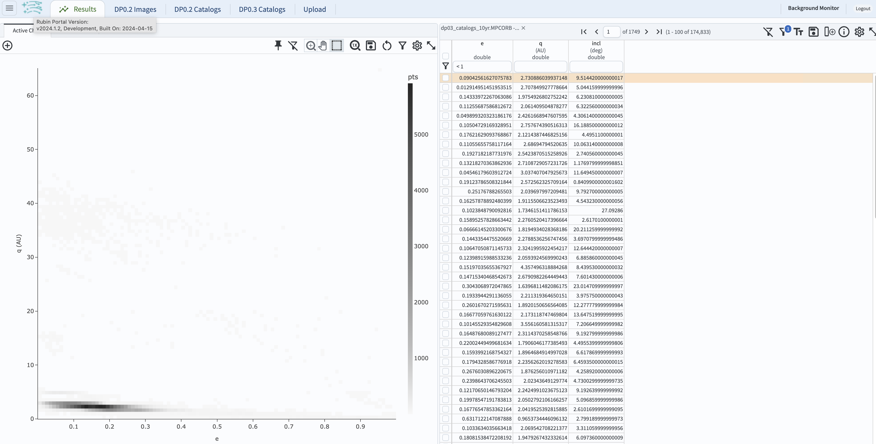
Figure 2: The view for the query with e < 1.#
1.6. Create a new column in the table, containing semimajor axis, a.
In the upper right column of the table panel, click on the icon to add a column (a tall narrow rectangle to the left of a + sign).
In the pop-up window to “Add a column”, set the “Name” to “a”, the “Expression” to “q/(1.0-e)”, the “Units” to “au”,
and the “Description” to “semimajor axis”.
Click “Add Column”, and see the new column appear in the table.
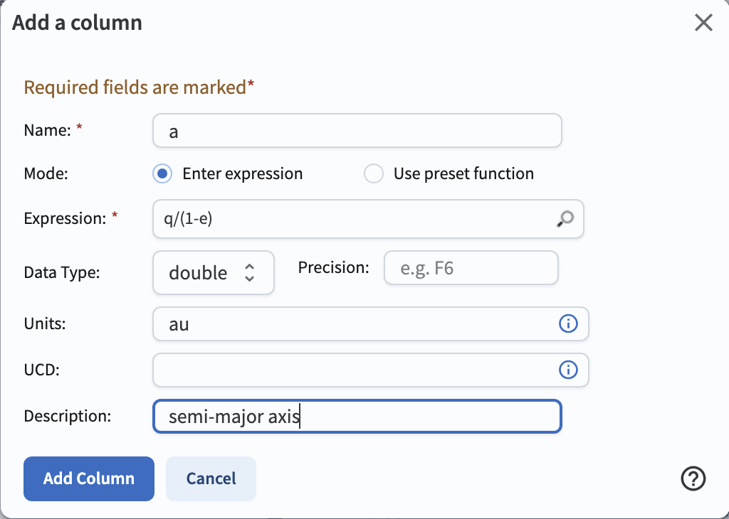
Figure 3: Screenshot showing the “Add a column” pop-up window.#
1.7. Create a scatter plot of inclination vs. semimajor axis. In the plot panel, click on the “+” sign the upper left side. This will bring up the “Add New Chart” pop-up window. Set the “Plot Type” to “Scatter”, the “X” to “a”, “Y” to “incl”. In the “Chart Options” dropdown menu, set the “X Min” to “0”, the “X Max” to 60, the “Y Min” to 0, and the “Y Max” to 80. Click “OK”.
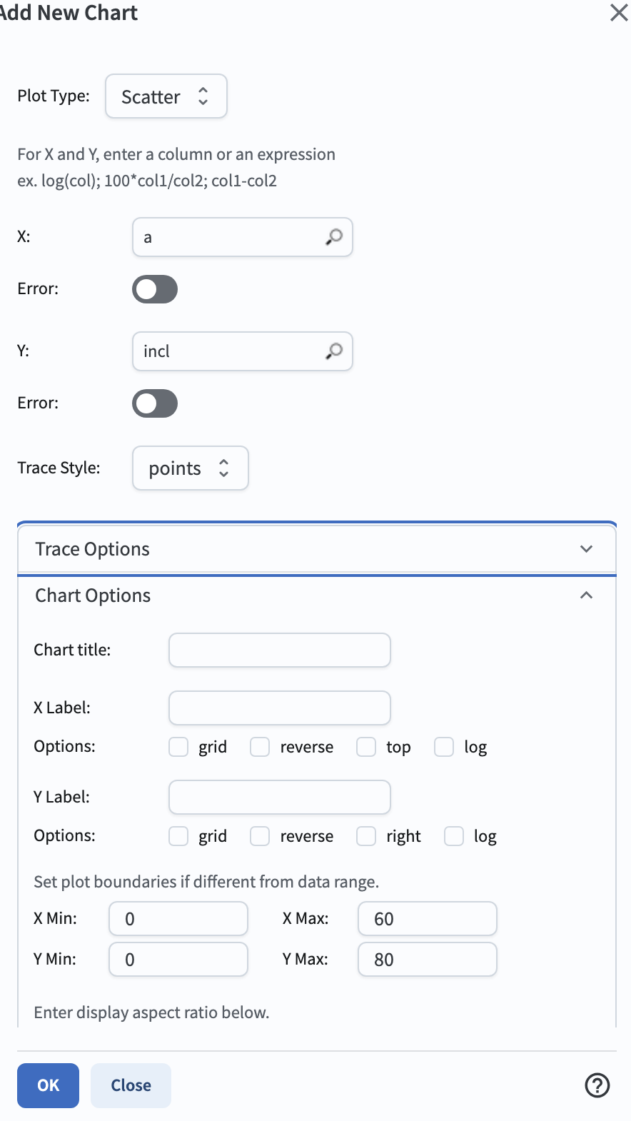
Figure 4: Screenshot showing how to create a new plot with these parameters.#
1.8. Delete the default plot by clicking on the blue cross in the upper right corner, so that only the newly-created plot appears (it should look like the plot below).
TNOs appear as a distinct population with a > 30.1 au in this parameter space.
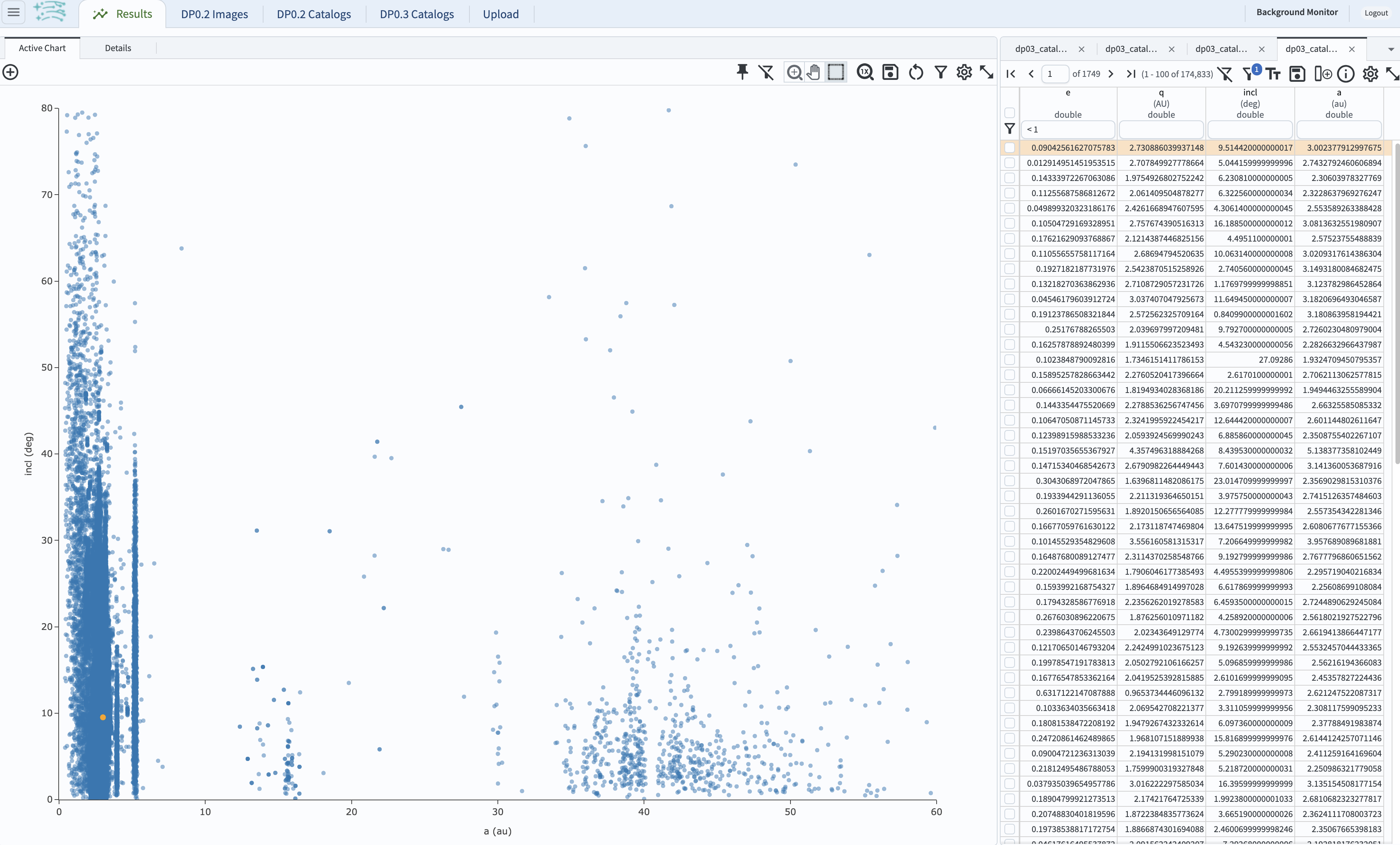
Figure 5: The population of TNOs has x-values greater than 30 au.#
1.9. Notice that in the plot above, the majority of objects returned by the query have semimajor axes less than 30.1 au. In fact, only about 800 of the moving objects from the query were TNOs. TNOs are at much larger distances from the Sun than Main-Belt Asteroids, which make them fainter and harder to detect and characterize, so fewer TNOs are expected to be detected than Main-Belt Asteroids. In the next step, a revised query will be used to only retrieve objects with semimajor axes greater than 30.1 au.
Step 2. Explore the properties of a population of TNOs#
2.1. Now isolate the population of transneptunian objects and further explore their properties. To study the properties of a larger sample of TNOs, return to the ADQL query interface by clicking on “DP0.3 Catalogs” tab, and clicking on “Edit ADQL” button.
2.2. Clear the ADQL query, and execute the query below, which is simiar to the one in Step 1.2 but includes only objects at a > 30.1 au.
Also include the absolute H magnitude mpcH which will be used in the derivation of TNO diameters in the subsequent step (2.6) below.
As TNOs aren’t the only solar system objects beyond Neptune, reject objects with mpcDesignation as
Long Period Comets (LPC).
SELECT e, incl, q, mpcH, mpcDesignation
FROM dp03_catalogs_10yr.MPCORB
WHERE q / (1 - e) > 30.1
AND SUBSTRING(mpcDesignation, 1, 3) != 'LPC'
2.3. Keep the “Row limit” to 200000, and click “Search”. This query will return 62,961 objects. The default plot in the results view will be a heatmap of inclination vs. eccentricity.
2.4. Plot the eccentricity of the orbit e as a function of the semimajor axis a.
This time (in contrast to Step 1.6 but accomplishing the same goal), calculate a from e and q via
setting appropriate plot parameters rather than creating another column in the right-hand table.
Start by clicking on the “+” sign on the left-hand panel to add a new chart.
2.5. In the “Add New Chart” pop-up window, select “Scatter” for the plot type.
Enter “q/(1.0-e)” for the X-axis, and “e” for the y-axis.
Increase the number of bins to 200 for both x and y to improve the resolution of the heatmap.
Expand the “Chart Options” and set the titles and labels as below.
Restrict the x-axis to 30 < a < 100 au.
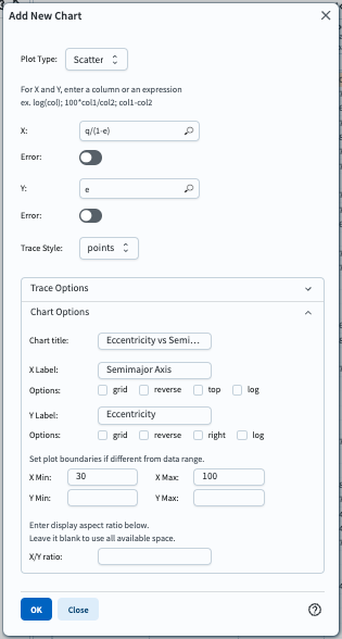
Figure 6: The plot parameters for the eccentricity vs. semimajor axis plot.#
2.6. Click on the “OK” button in the “Add New Chart” window, and view the plot (see below). Delete the default plot of inclination vs. eccentricity as it is not needed.
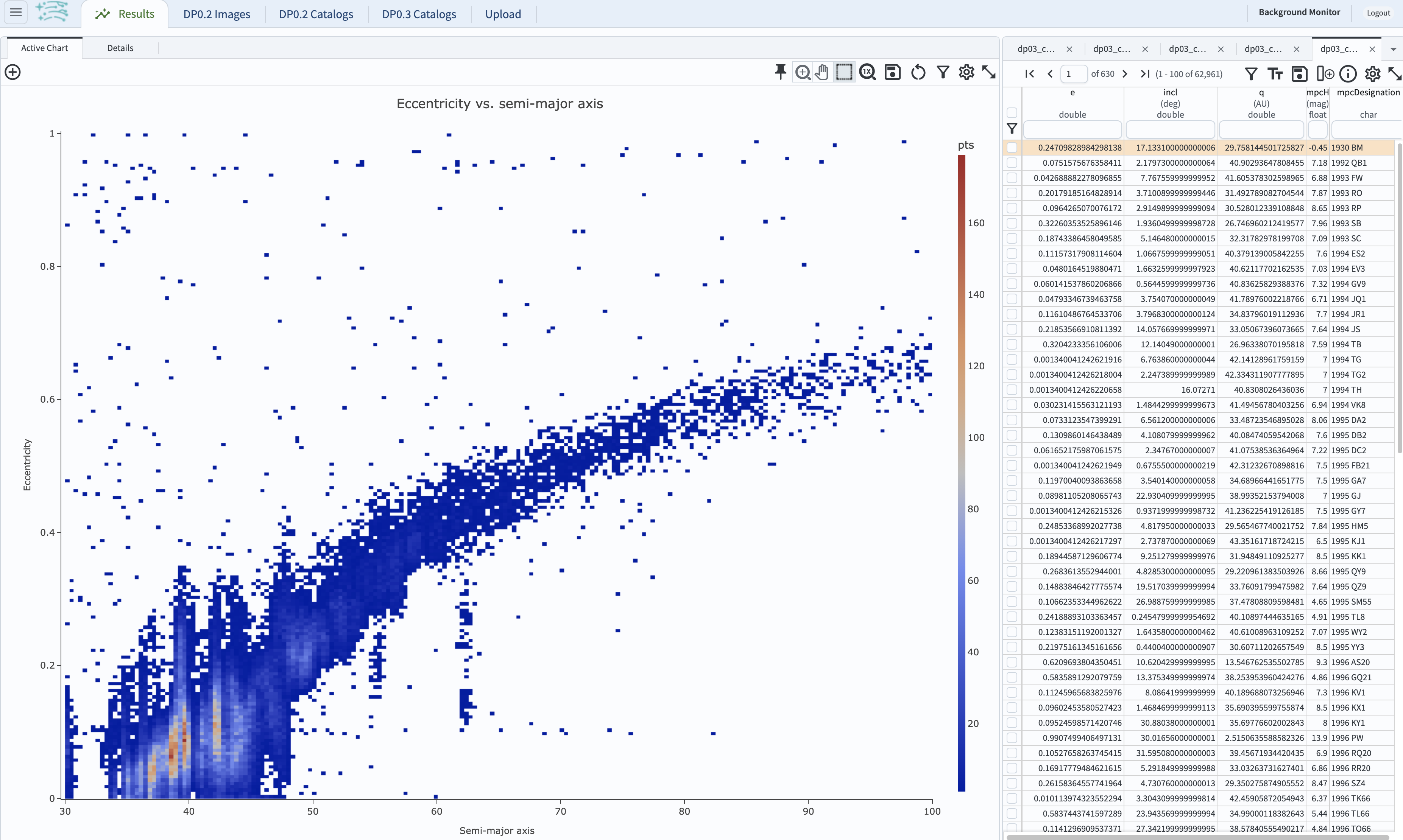
Figure 7: The plot of eccentricity vs. semimajor axis of transneptunian objects (TNOs).#
2.7. Multiple sub-populations are apparent in the above plot.
The majority of the objects have low eccentricity (e < 0.3) and a semimajor axis of about 30 to about 50 au.
There are several sub-populations of transneptunian objects, such as the classical, resonant, scattered-disk, and detached sub-populations.
A full review of all TNO sub-populations is beyond the scope of this tutorial.
2.8. Estimate the diameters of the objects using their absolute H magnitudes.
Where H is the absolute H magnitude (column mpcH), and A is the albedo, the diameter \(d\)
in kilometers is \(d = 10^{(3.1236 - 0.5 \times log(A) - 0.2 \times H)}\).
This tutorial adopts an albedo value of 0.15 (as is commonly adopted, e.g., Vilenius et al. 2012),
with which the expression reduces to \(d = 10^{(3.536 - (0.2 \times H))}\) km.
Click on the “add column” icon.
Enter D in the “name” field, power(10,(3.536 - 0.2 * mpcH)) in the expression field, “km” as the units, and “diameter” as the description as below.
Click the “Add Column” button.
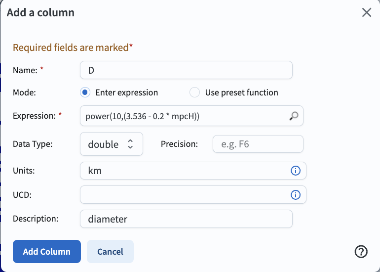
Figure 8: How to add a new column containing the estimated diameter.#
2.9. Plot the distribution of estimated diameters in log-space. Click on the “+” sign in the pop-up window, click on “Add New Chart,” select “Histogram”, and enter the parameters as below.
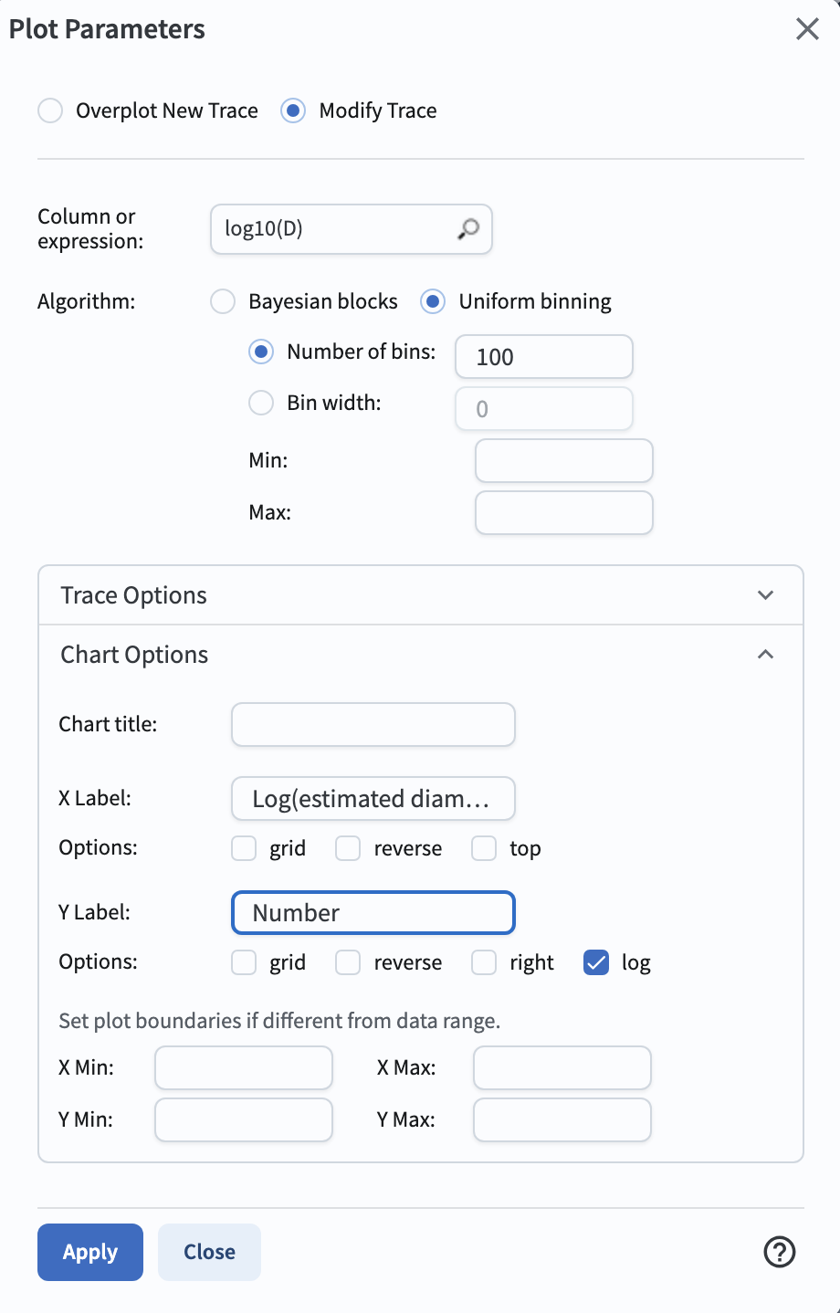
Figure 9: The plot parameters for the distribution of estimated diameters.#
2.10. Click on the “OK” button. This will result in the plot showing the distribution of estimated diameters.
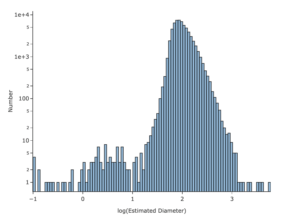
Figure 10: The distribution of estimated diameters.#
2.11. Notice that the tail of the distribution extends to very small diameters. This is suprising, as detecting kilometer-sized objects at the distance of Neptune should be quite challenging. This illustrates, in part, some of the shortcomings of the assumptions (such as albedo) which were used to estimate the diameters. See also the first exercise for the learner in Step 6.
Step 3. Find and explore a well-observed TNO#
3.1. Return to the RSP TAP Search form by clicking on the ‘DP0.3 Catalogs” tab. Navigate to the ADQL interface by clicking on the “Edit ADQL” button.
3.2. To identify a distant Solar System object with a large number of observations, enter the query below.
This query joins the MPCORB table with the DiaSource table in order to retrive the number
of detections: the count of the number of DiaSource table rows for a given solar system object,
each of which has a unique ssObjectId.
This query also constrains the semimajor axis to between 30 and 100 AU,
and constrains the ssObjectId to return a random subset (similar to Step 1.2).
SELECT mpc.ssObjectId, COUNT(ds.ssObjectId), mpc.e, mpc.q
FROM dp03_catalogs_10yr.MPCORB AS mpc
JOIN dp03_catalogs_10yr.DiaSource AS ds ON mpc.ssObjectId = ds.ssObjectId
WHERE mpc.ssObjectId < -700000000000000000
AND mpc.q > 30 * (1 - mpc.e)
AND mpc.q < 100 * (1 - mpc.e)
GROUP BY mpc.ssObjectId, mpc.e, mpc.q
3.3. Click on “Search”. This search might take up to a minute. The query returns 12,589 objects.
3.4. The default plot generated for the query above shows the first two columns against each other, ssObjectId and COUNT,
which is not a particularly useful plot aside from showing that the number of detections for the most oft-detected objects in the outer Solar System
is in the thousands.
Click twice on the COUNT2 column header to order the entries by descending count and identify the most oft-detected outer Solar System object.
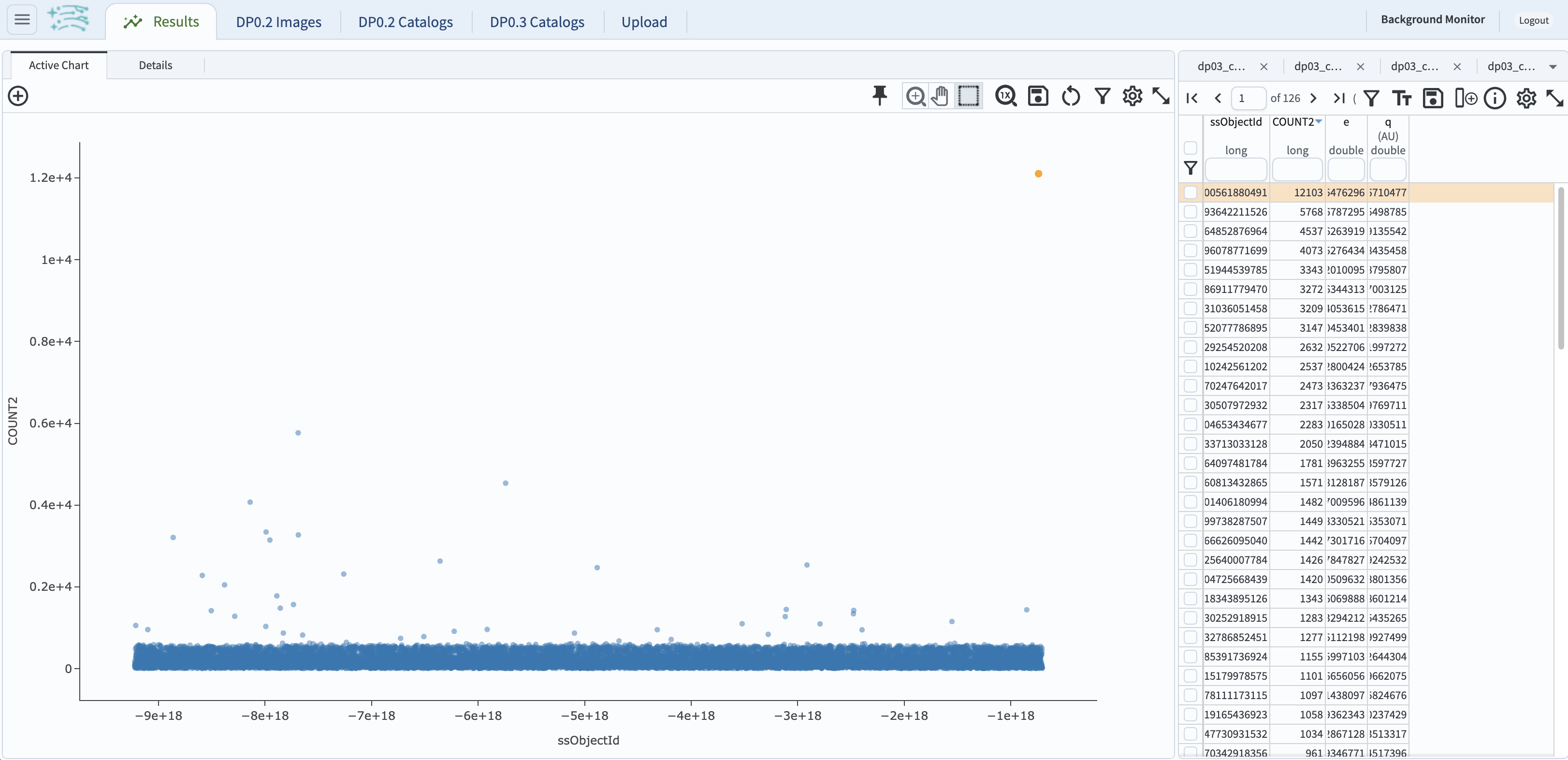
Figure 11: The default results view from the ADQL query above.#
3.5. Continue with the object with the largest number of observations: ssObjectId = -735085100561880491, which was detected 12,103 times.
Its modest eccentricity of 0.152 implies that this is a TNO (unlikely to be a comet).
3.6. Return to the ADQL query interface and use the following statement to retrieve the sky coordinates, magnitudes, filter (band), and time of observations (midPointMjdTai) for the oft-observed TNO with ssObjectId as above.
SELECT ra, dec, mag, band, midPointMjdTai
FROM dp03_catalogs_10yr.DiaSource
WHERE ssObjectId = -735085100561880491
3.7. The default results view will show the “Coverage” map at upper left. In the future, with real LSST data, this map would have an underlay of the LSST deeply stacked image. Since DP0.3 has no images, the “Coverage” map only shows the overlay of RA vs. Dec, which is redundant with the default plot. Click on the “hamburger” icon (three horizontal lines) on the upper left, and click on the “Results Layout” box. In the left-hand window, select the “Coverage Charts Tables” box (at the bottom). In the window on the left, click on “Active Chart” tab.
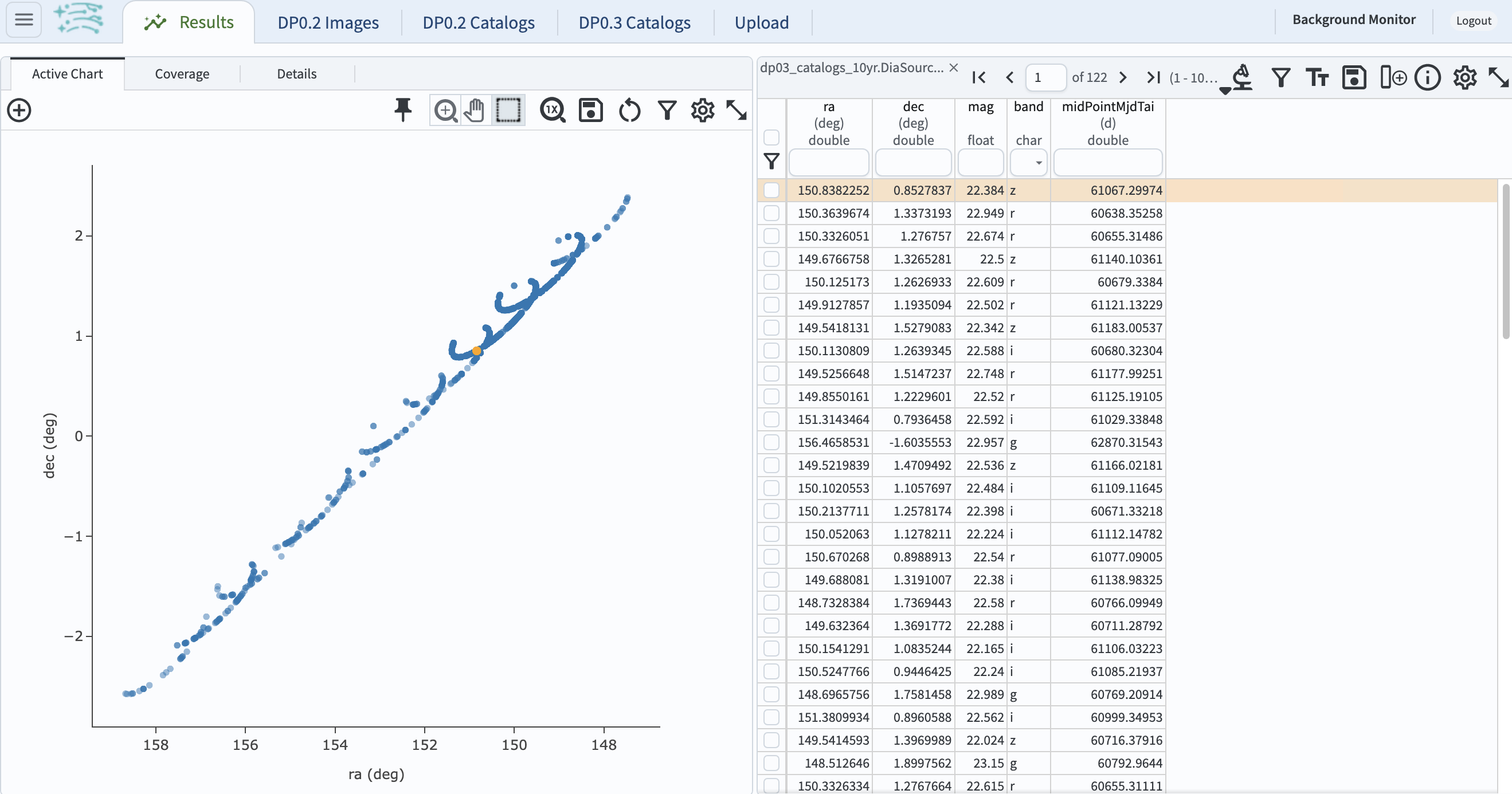
Figure 12: The “Charts Tables” results view of the selected object illustrating its movement on the sky as seen from the Earth.#
3.8. Set the color of individual points to represent the time of the observation to better illustrate how the object moves across the sky as a function of time. In the plot panel, click on the “Settings” icon (a gear) to open the “Plot Parameters” pop-up window. Under “Trace Options”, for “Color Map” enter “midPointMjdTai” and for “Color Scale” enter “Rainbow”. Then click “Apply” and “Close”.
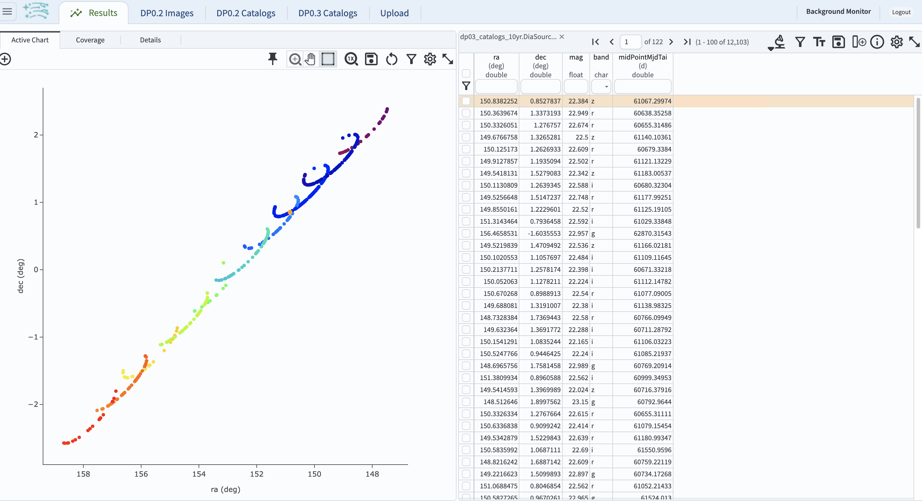
Figure 13: Purple color corresponds to earlier observtations, and the red color corresponds to later observations.#
3.9. In the plot above, the 10 loops in the object’s path on the sky is a result of Earth’s orbital period and the 10-year LSST duration. As described in the introduction, this particular TNO was detected by LSST over ten thousand times because it happened to be in a deep drilling field. This will not be the case for the majority of solar system objects.
Step 4. Plot the time-domain quantities for the TNO#
Note that no time domain evolution in object brightness was included in the DP0.3 simulation (e.g., rotation curves for non-spherical objects, outgassing events). All changes in the brightness of DP0.3 objects with time are due to changes in the distance and phase angle from Earth.
4.1. Return to the search form and execute the following ADQL query to retrieve the r-band magnitudes, phase angles, heliocentric and topocentric distances, and time of the observations for the TNO explored in Step 3.
SELECT ds.midPointMjdTai, ds.mag, ds.band,
ss.phaseAngle, ss.topocentricDist, ss.heliocentricDist
FROM dp03_catalogs_10yr.DiaSource AS ds
JOIN dp03_catalogs_10yr.SSSource AS ss ON ds.diaSourceId = ss.diaSourceId
WHERE ss.ssObjectId = -735085100561880491
AND ds.band = 'r'
4.2. The default plot will have the r-band magnitude as a function of time.
In the right-hand panel, click the “Active Chart” tab.
Click on the “+” sign in the plot panel to add a scatter plot showing the phase angle as a function of time.
For the x-axis, use midPointMjdTai - 60000 to show more clearly the timescales between observations.
4.3. As mentioned above, the simulated Solar System data does not include any time-varying features. The changes in apparent magnitude are due to the object changing in phase angle and distance from Earth as a function of time. Add two new scatter plots showing the r-band magnitude as a function of phase angle and as a function of topocentric (Earth-centered) distance, as is shown below. The results view for four plots automatically reconfigures to a two-by-two grid. Notice how the magnitude is a monotonic function of phase angle and distance, but not time.
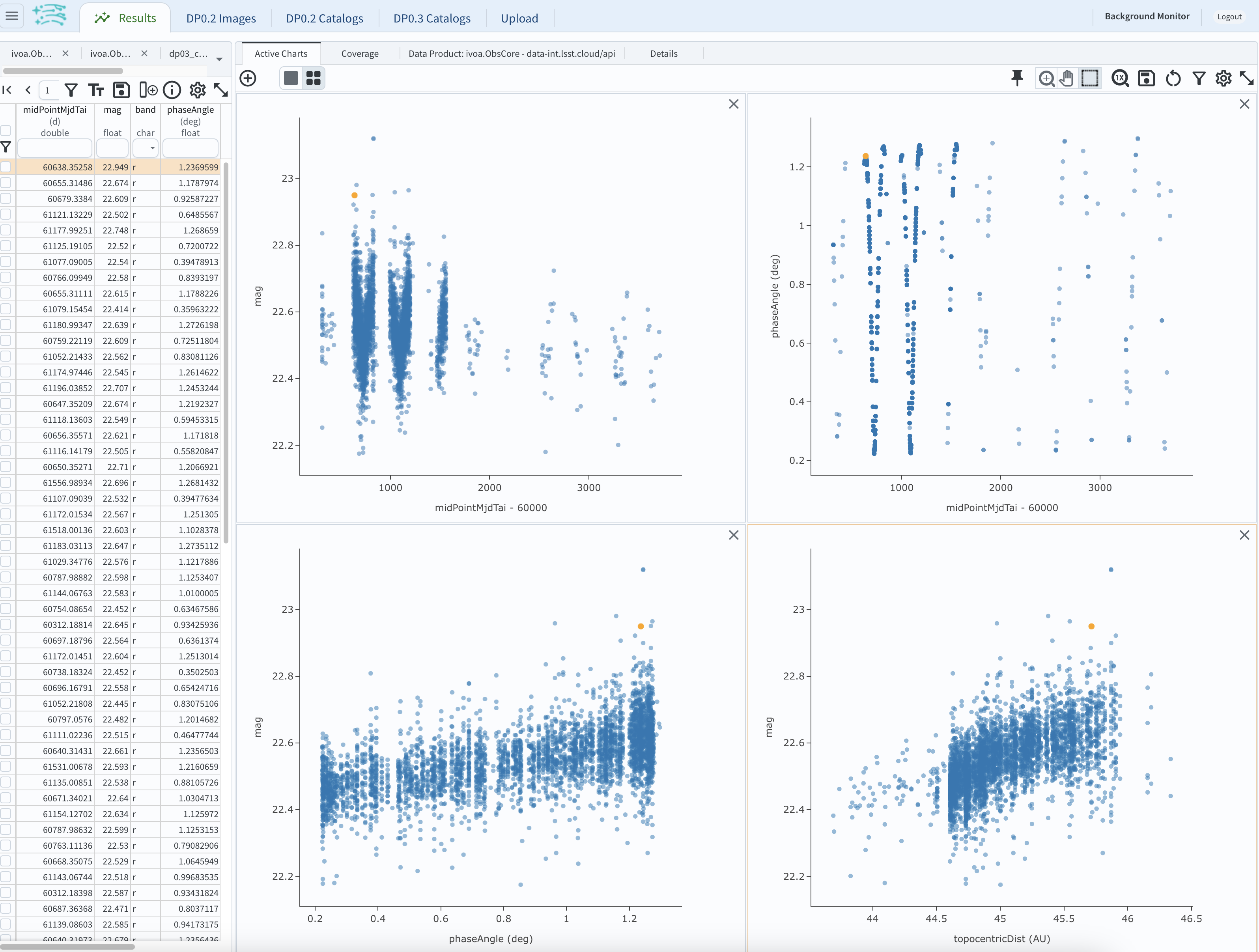
Figure 14: Four plots demonstrating that the apparent magnitude depends on phase angle and distance from Earth.#
4.4. Plot the topocentric and heliocentric distances of the object as a function of time already retrieved in Step 4.1.
First, delete all but one of the plots prepared in Step 4.3 by clicking on the blue X in the upper right-hand part of any three of the four plot panels to make space for new plots.
Then add a pair of new scatter plots that show topocentricDist and heliocentricDist
as a function of midPointMjdTai - 60000.
Then delete the remaining old plot so that only the two new plots are displayed.
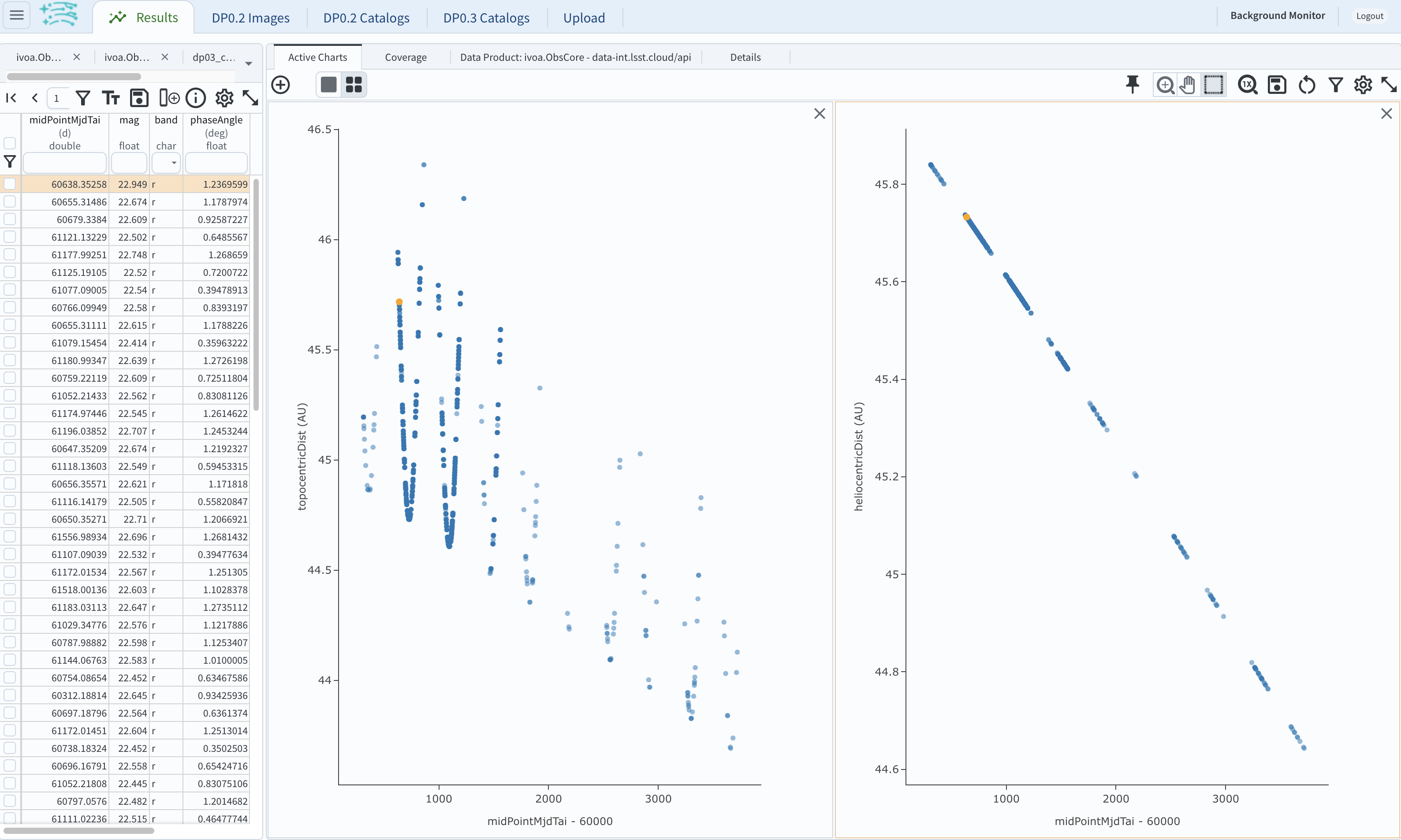
Figure 15: Heliocentric and topocentric distance of the TNO as a function of time.#
4.5. The left plot shows the periodic change of the topocentric distance with time resulting from the Earth’s motion around the Sun - a different view of the same effect seen in Step 3. The right plot shows that this object is on a slightly inbound trajectory with respect to the Sun.
Step 5. View the 2-D projection of the TNO’s orbit to visualize its 3-D trajectory#
5.1. The goal of Step 5 is to visualize the 3-D trajectory of the well-observed transneptunian object, via viewing the projections of its 3-D heliocentric and topocentric distances as a function of time into 2-D. Navigate to the ADQL query interface. Execute the query below to extract the heliocentric and topocentric X, Y, and Z distances of the TNO needed to visualize its trajectory.
SELECT heliocentricX, heliocentricY, heliocentricZ,
topocentricX, topocentricY, topocentricZ, ssObjectId
FROM dp03_catalogs_10yr.SSSource
WHERE ssObjectId = -735085100561880491
5.2. The default plot will be the heliocentric Y distance as a function of heliocentic X distance as in the screenshot below. Note that the object moves slowly in heliocentric coordinate X as well as in Y (by a comparison to, e.g., Earth’s motion), covering only a few au in 10 years. This is expected given its distance from the Sun.
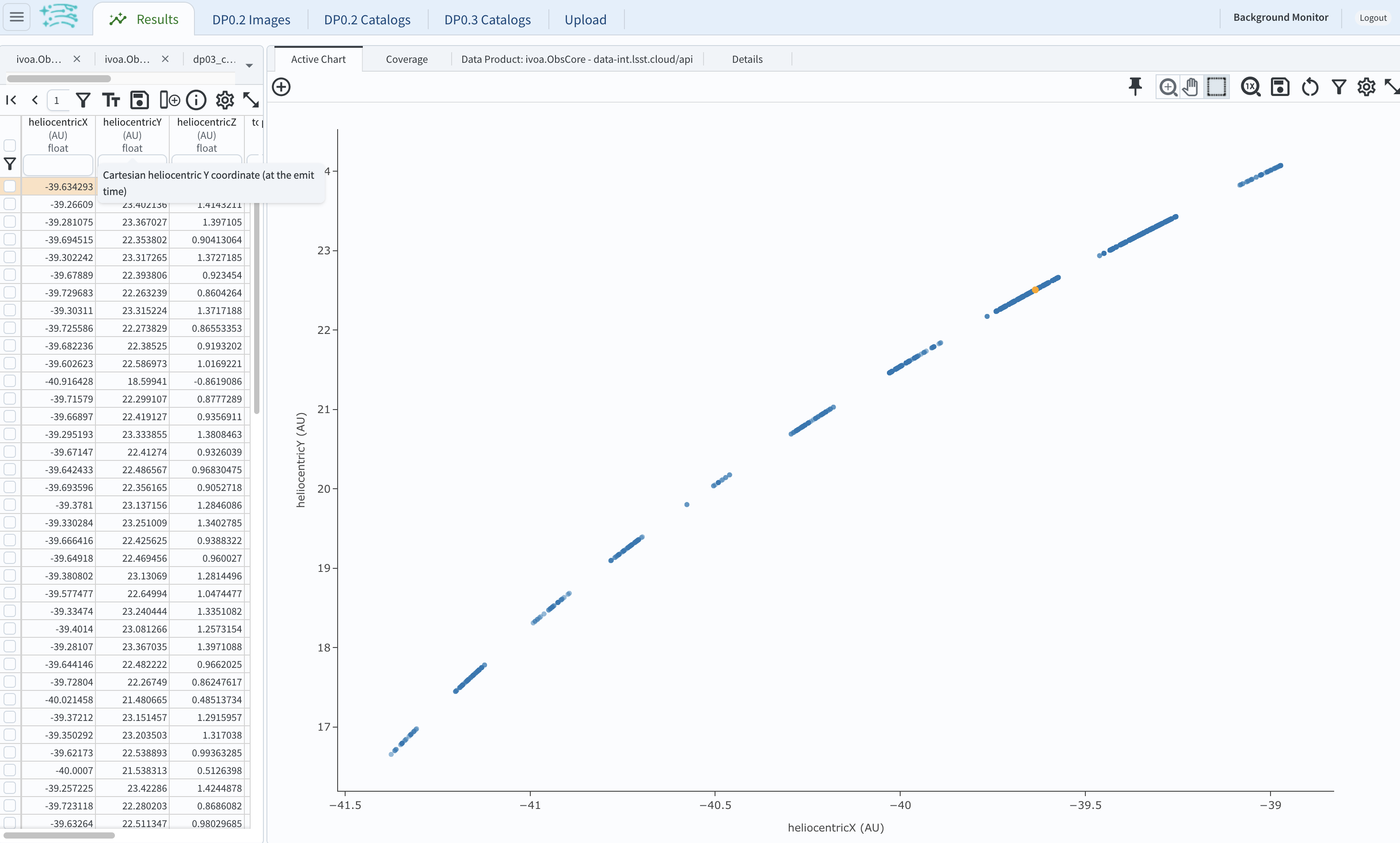
Figure 16: Heliocentric Y vs. X distance of the transneptunian object.#
5.3. Now plot the heliocentric Z distance as a function of heliocentric X distance. Click on “+” button to add a new chart.
Select heliocentricZ for “y” and heliocentricX for “x”.
Click on “Apply” or “OK.”
5.4. Observe that the object’s trajectory is not constant in Z, which means that its orbit is not in the plane of the Ecliptic during the simulated Rubin observation, but the object does pass through the ecliptic plane when Z = 0.
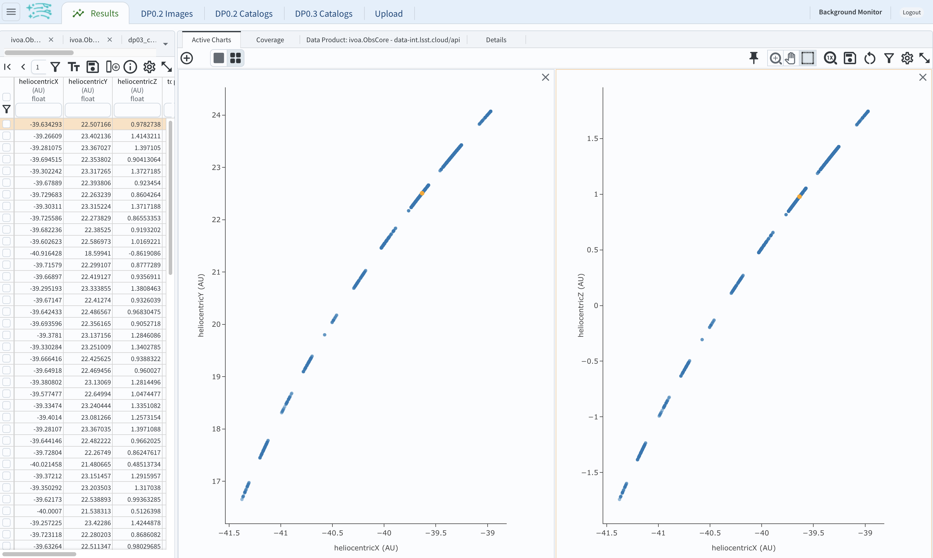
Figure 17: Heliocentric Y vs. X distance as well as helliocentric Z vs. X distance of the transneptunian object as a function of time.#
5.5. Next, plot the topocentricY vs. topocentricX and topocentricZ vs. topocentricX distances.
On the same screen with the generated plots from the previous two steps, click on the “+” button to add a new chart.
First, select topocentricY for “y” and topocentricX for “x”. Click “OK.”
Next, click again on “+” button to add a new chart. Select topocentricZ for “y” and topocentricX for “x”, and click “OK.”
The result shows the position of the TNO on the sky as a result of Earth’s orbital motion.
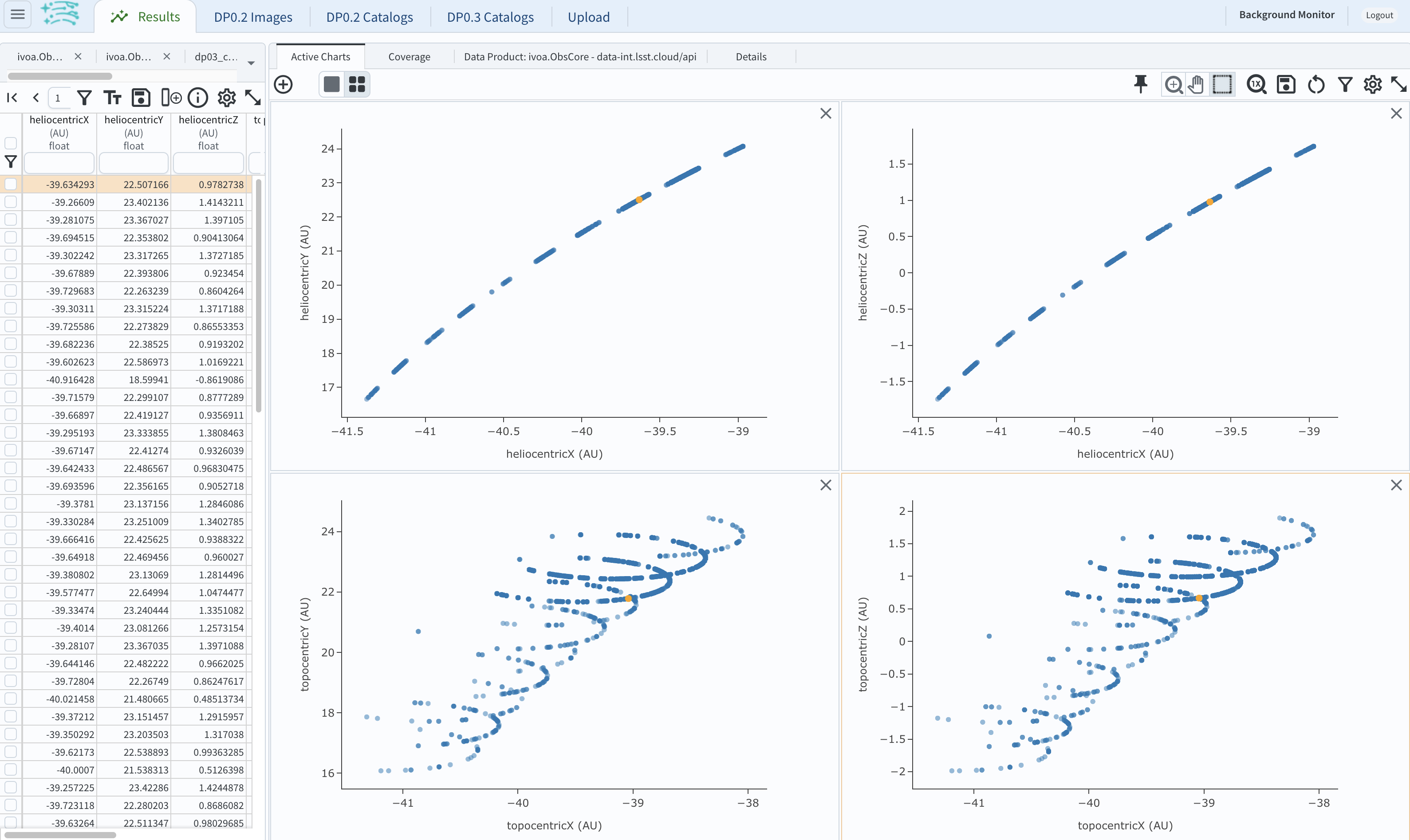
Figure 18: Visualization of the 3-D TNO trajectory by viewing the 2-D projections of its trajectory as measured from the Sun (top two plots) and the Earth (bottom two plots).#
Step 6. Exercises for the learner#
6.1. In Step 2, some of the sizes of the TNOs were on order one kilometer, quite small for objects at the distance of Neptune. However, objects with high eccentricities could come closer to Earth, and be detected despite their small size. For the objects returned by the query in Step 2, plot the eccentricity vs estimated diameter. Explore whether some of the smallest objects have large eccentricities.
6.2. Plot the histogram of the number of visits to the Solar System objects in the dp03_catalogs.SSObject for objects observed more than 1000 times.
6.3. Repeat the steps 4 and 5 for another object with a large number of observations (say another one with numObs > 2000).
Note that objects with large numbers of observations were already identified in Steps 3.1, 3.2, and 3.3.