05. Using user-supplied catalogs in DP0.3 (beginner)#
Contact authors: Christina Williams and Melissa Graham
Last verified to run: December 22, 2023; update to reflect the new user interface (UI) started on May 9 2024
Targeted learning level: Beginner
Introduction#
This tutorial demonstrates a functionality of the Portal aspect for user-uploaded tables and their use in queries for DP0.3 (not available for DP0.2 yet).
This tutorial assumes the successful completion of the beginner-level DP0.3 Portal tutorials, and uses the Astronomy Data Query Language (ADQL), which is similar to SQL (Structured Query Language). For more information about the DP0.3 catalogs, tables, and columns, see the DP0-3-Data-Products-DPDD.
Step 1. Upload a user-supplied table of coordinates for use in cone searches#
The scientific scenario used for this demonstration is to answer the question of whether LSST detected a moving object which, based on its known orbit, was expected to appear at given coordinates.
The list of expected coordinates and dates is provided in a file with nine rows (i.e., nine expected locations and times), with the format expected for user-uploaded tables: column names in the first row with no # symbol at the start of the row. The list contains columns of right ascension, declination, and modified julian date (ra, dec, and mjd).
1.1. Log into the Rubin Science Platform at data.lsst.cloud and select the Portal aspect. Click on “DP0.3 Catalogs” tab on top of the window. The Table Collection (Schema) tab should default to “dp03_catalogs_10yr”. Select “dp03_catalogs_10yr.DiaSource” table in the right-hand tab.
1.2. In the “Enter Constraints” box, check only the box to the left of the “Spatial” section (uncheck the other two if checked), and click on the “Multi-object” button. A window will pop up to allow the upload of a text file containing ra and dec coordinates for sources of interest. The format of this catalog must be one of those listed (IPAC, CSV, TSV, VOTABLE, or FITS table format). For this example, we prepared a file which is is an ascii catalog with columns of RA and Dec in tab separated format (TSV). The name of the file is portal_tut05_useruploadcat1.cat. Other columns can also be present in the file, but note that the header names and columns must not have multiple spaces or tabs between them. The uploader is agnostic about header labels, because you can choose which columns to use later (i.e. ra and dec do not necessarily have to be labeled as such). Make sure to remove any pound sign (#) from the header before uploading.
1.3. Download the file to your computer using the link to file in GitHub containing the catalog. If you are a novice using GitHub - click on this link which will take you to the GitHub repository containing the file, and click on the “download” tab (an arrow pointing down into an open box).
1.4. Upload the file from your computer to the Portal. If you haven’t done so in Step 1.2 - click on the “Multi-object” button, which will result in a pop-up window as illustrated below. Click on “upload file”. Either drag the file into the window, or click the choose file button and navigate to and select the file. After loading, hit the blue Load Table button.
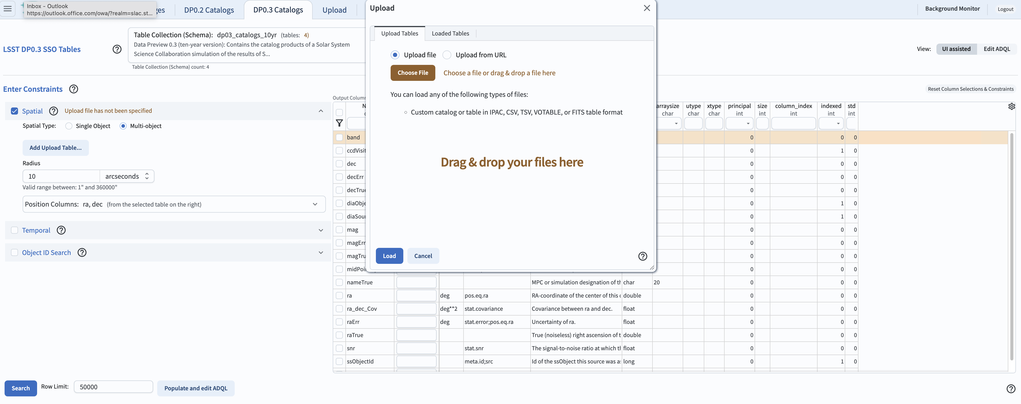
Figure 1: A screenshot of the Portal screen - ready to upload a table - with the “Upload” pop-up window.#
1.5. After uploading, the pop-up window will show a list of the columns it found, named according to the header. Make sure that the ra and dec columns in the file are labeled “ra” and “dec” and are displayed in the list. Then click the “Load Table” button. If the table loaded the ra and dec correctly, the table filename should be displayed next to “Change Upload Table”, and listed next to “Position Columns” should show “ra, dec (from the uploaded table)”.
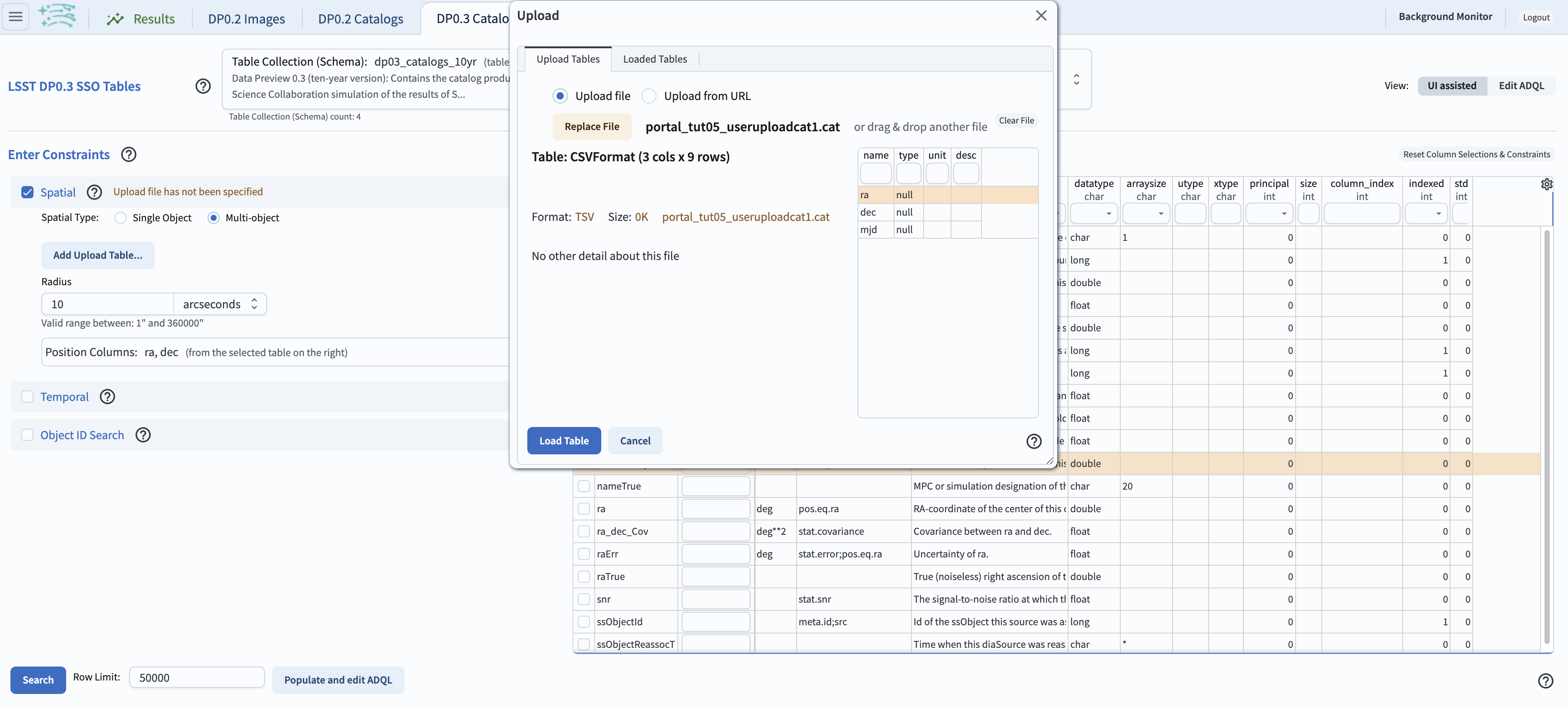
Figure 2: A screenshot of the search query if the user-supplied catalog has uploaded and identified the correct columns for search.#
1.6. Still under the “spatial” constraint inputs but under the “Radius” box, click the arrow next to “Position Columns (from the selected table on the right)” and a sub-menu will lower. Here, the user must indicate which of the DP0.3 catalog columns to use for the spatial matching (i.e. from among the row names listed right below “output column selection and constraints”). If the header names are recognized as ra and dec then they may auto-populate into the “Lon Column” and “Lat Column” boxes. If they do not (e.g. the header uses different labels than ra/dec), then click the arrow next to “position columns” and enter “ra” into the “Lon column” and “dec” into the “Lat column”. Leave the search radius at the default of 10 arcseconds.
1.7. For a first look, ignore the “Temporal” constraint and make sure the box is unchecked. Click the “Search” button. This search will return whether any moving object was ever detected within a search radius of 10 arcseconds of these locations in the uploaded table. Select the format of the display by clicking on the “hamburger” icon (three horizontal lines on the upper left), and select the “Coverage / Charts / Tables” in the “Results Layout” box. (Note: leaving the “Row Limit” set to 50000 during the search will prevent the search from taking too long. This example returns fewer than the row limit.)
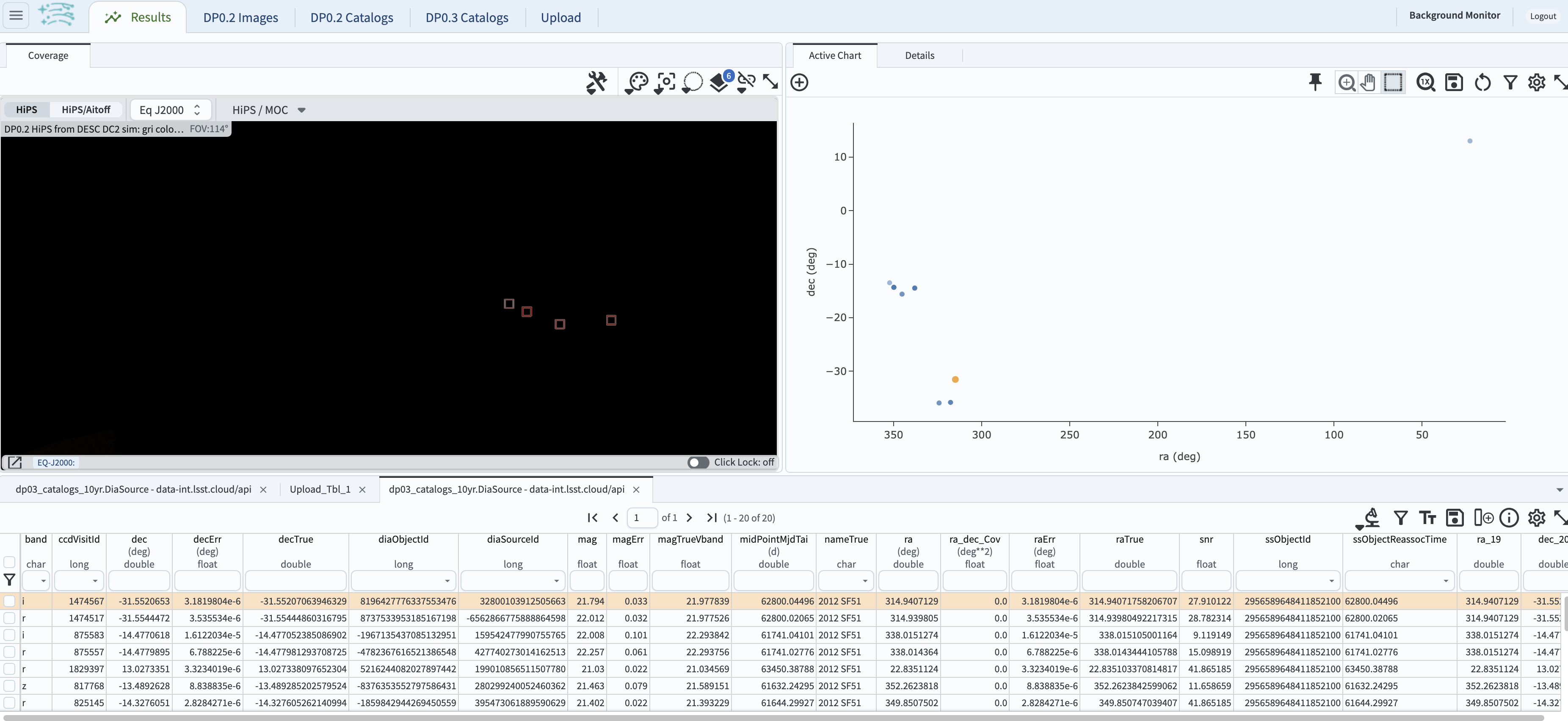
Figure 3: A screenshot of the search query result, showing the multiple observations of 3 solar system objects from the user-uploaded table - those can be seen as the clustered points.#
1.8. Now, click the DP0.3 Catalogs tab to return to the search query page. For a second example, now also set a “Temporal” constraint for the search by clicking the box (leaving the Spatial box also checked). This example demonstrates how to know if there were moving objects identified in the survey at these coordinates on a specific night (for this example, pick a day for which it is known that this is the case from the mjd column of the user-supplied catalog). Click the “Temporal” box and make sure the “temporal column” box contains “midPointMjdTai” (referring again to the column in the DP0.3 DiaSource table to use for temporal matching). Click the MJD specification and enter an MJD range (start date 62000 and end date 63000, a range that we know our sample objects was observed in the catalog). The search returns an observation of 4 unique solar system objects, one of which is observed twice during the MJD range.
1.9. It can be useful to save the search for later. In this case it can be automated with search query commands that are output by the “populate and edit ADQL query” button. Repeat Step 1.7, but instead of hitting the “search” button, hit the “populate and edit ADQL” button on the bottom right. This will navigate to the “advanced ADQL interface” where the reproducible search code snippet to perform the search (e.g. in a notebook) is shown on the right. In the schema browser on the left, the name of the user-supplied catalog is displayed as a searchable table under TAP_UPLOAD.
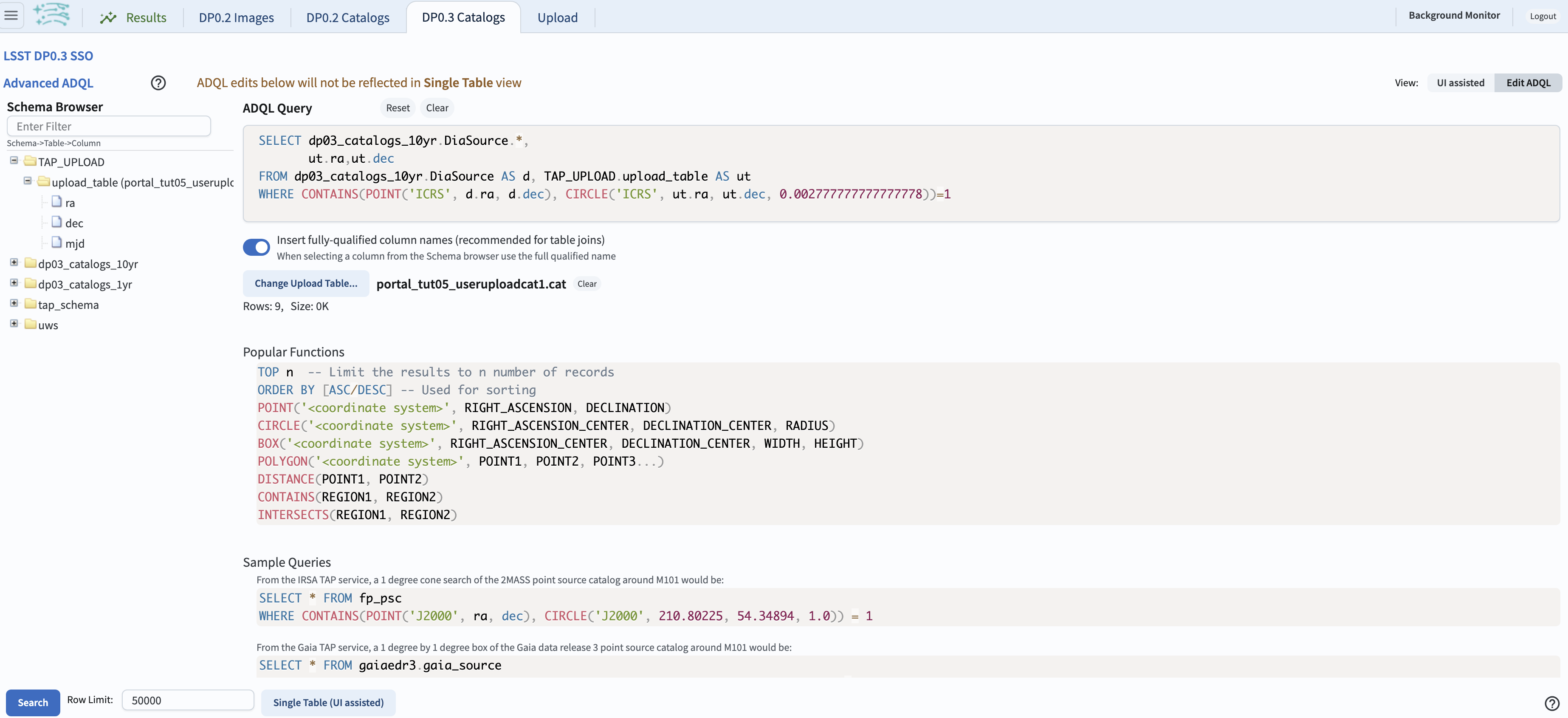
Figure 4: A screenshot of the “advanced ADQL interface” which shows the ADQL search corresponding to the one entered into the portal user interface, for future use with a TAP service.#
Step 2. ADQL table join with user-uploaded list of ssObject IDs#
This section demonstrates how to upload a user-supplied table and join it with a DP0.3 table.
In this scenario, a list of identifiers (ssObjectId) for moving objects has been assembled by the user and stored in a file (one column, two rows of data, i.e. two independent objects).
2.1. Return to the main DP0.3 Catalogs tab to go back to the search interface by clicking the “UI assisted” buttom on the top right, and unclick the spatial and temporal boxes. Make sure the box labeled “Object ID search” is clicked. Download to your computer a sample catalog named portal_tut05_useruploadcat2.cat prepared by us for this exercise (from this ` link <lsst/dp0-3_lsst_io>`_) - using the procedure in Step 1.3. Click on the “Change Upload Table” and replace the table you loaded in the Step 1 with the one you just uploaded to your computer. Click on “Load Table” button. Clicking the down arrow in the “Object ID Search” box, and clicking the “Load object IDs from a table” button will then give access to the upload button to supply a catalog containing IDs. Click the “Add Upload Table” button and navigate on your machine to the file containing the catalog of IDs to be used. A pop-up window will appear, where you can upload the file. Then click on “Load” button in the pop-up window. To use this feature, the IDs listed must correspond to a Rubin table ID (in this case, the ssObjectId).
2.2. In the “Object ID Search” box, click the arrow in the box next to “Uploaded Object ID”. Click the magnifying glass near “ID” and in the window that pops open, select the “ssObjectId” header keyword from the table that was uploaded, and hit OK. The object ID box should now contain ssObjectId (or whatever header label is used for ID in the user suppled catalog).
2.3. Now go below to the “object ID (from table)” section and click the arrow to open the box that allows one to specify which type of ID in the catalog to the right to match on. The default Object ID type that is listed will be based on the DP0.3 table that is selected in the menu above (LSST DP0.3 SSO Tables), which is by default the DiaSourceId from the DiaSource Table. But this exercise will instead match on ssObjectId, which will retrieve information for specific solar system bodies identified by their unique identifier. Click the magnifying glass to open a navigation window to choose which ID from the DP0.3 table to use, and select ssObjectId.
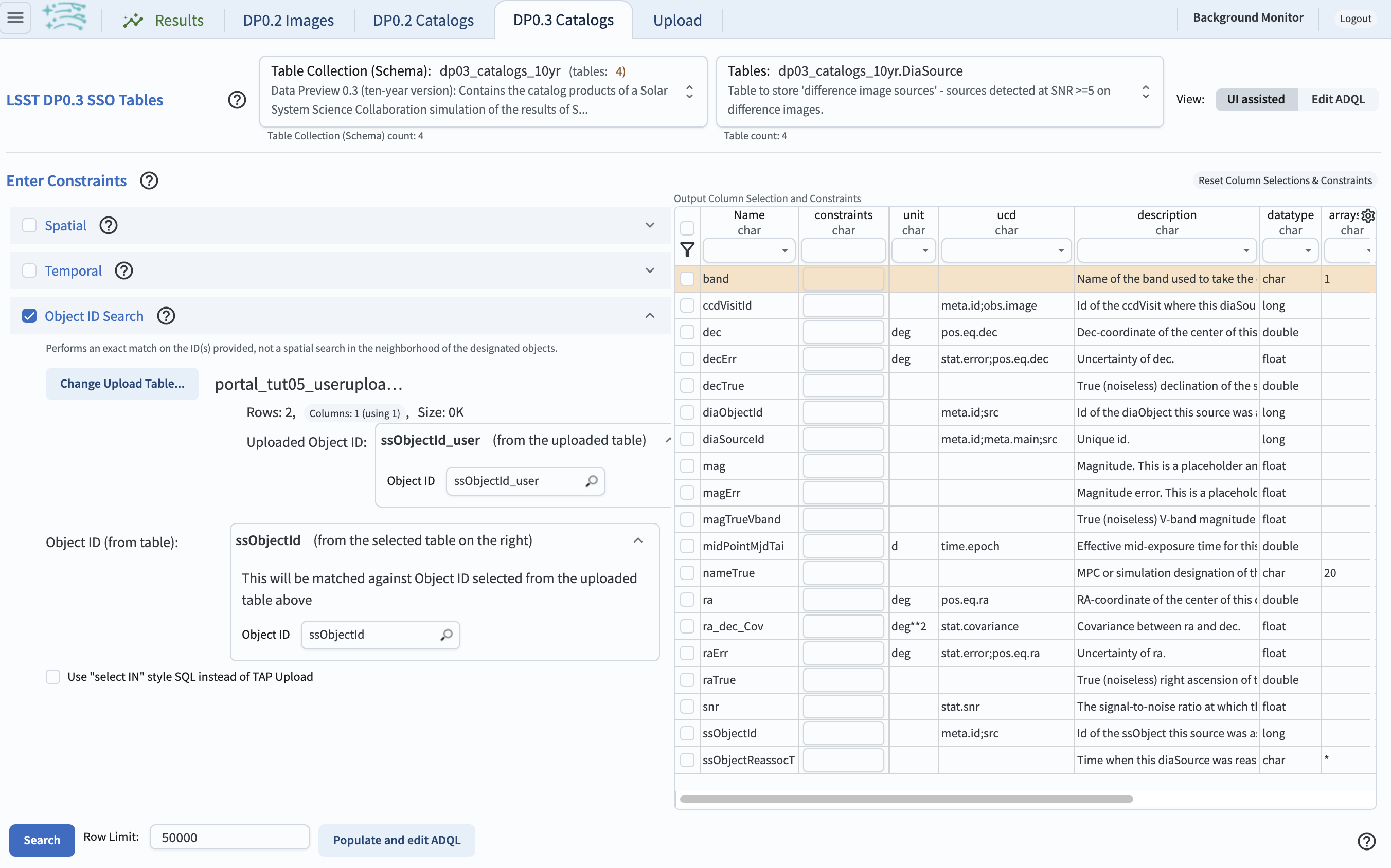
Figure 5: A screenshot of the portal user interface demonstrating the view after correctly uploading a table of IDs and identifying how to match to the DP0.3 catalog.#
2.4. Hit the search button. Note: searching on IDs without a spatial constraint included can take several minutes since the database is parsed by celestial coordinates. This example searchs for 2 unique ssObjects from the user-supplied table, and the output looks as in the below screenshot. It will return the moving source observations for both sources over the 10yr survey lifetime. To view each object separately, go to the table column ssObjectID and click the downward arrow. This will pop up a window listing the unique ssObjectIds. Clicking the box next to an ssObjectId and clicking “filter” will plot the data for that single object.
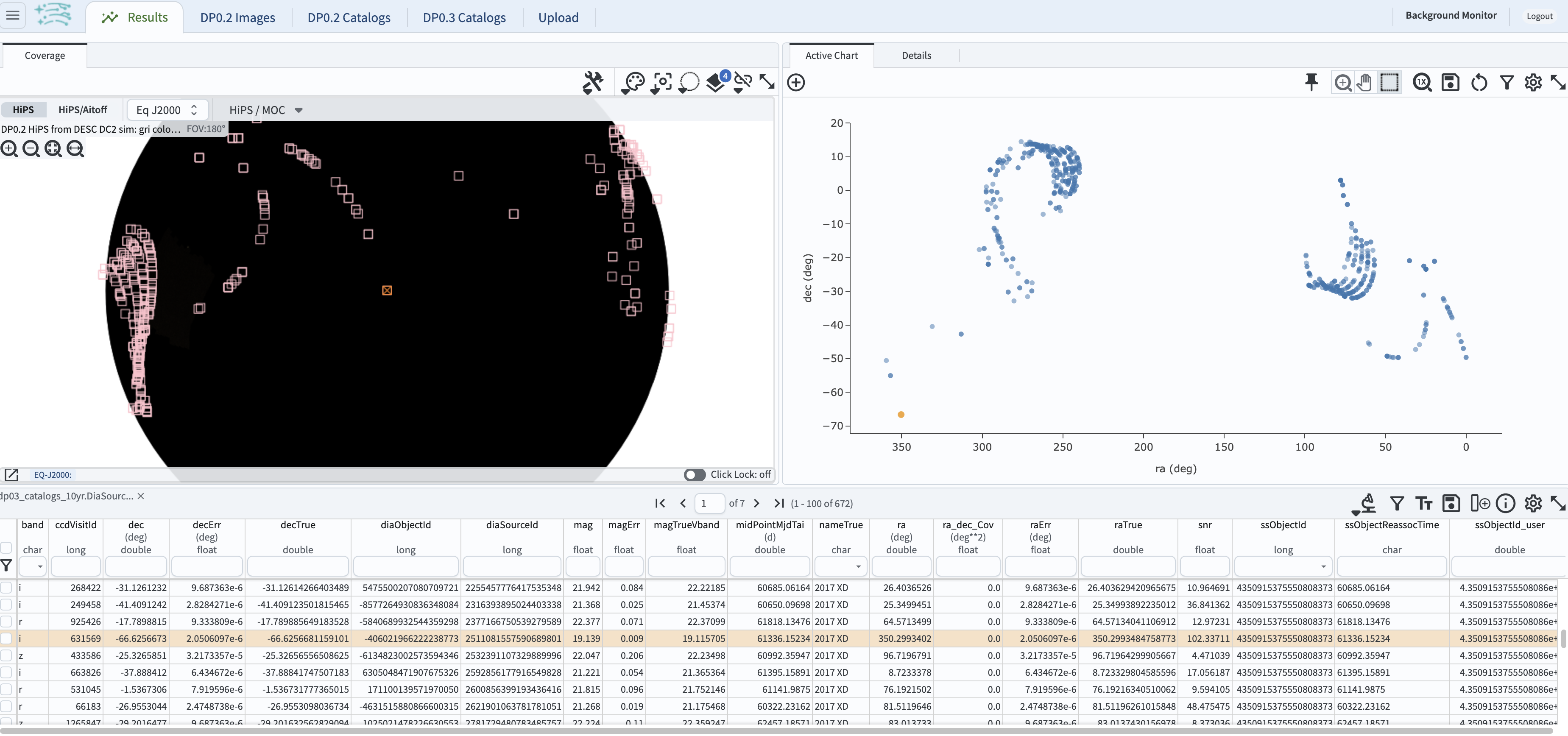
Figure 6: A screenshot of the portal user interface after searching the 10 year catalog for 2 unique solar system objects based on their ssObjectIDs.#
2.5. Now use the ADQL interace to perform the join on ssObjectID between the uploaded table and the DP0.3 table. Start over at the main portal interface by clicking the “DP0.3 Catalogs” tab and click the upper right botton called “Edit ADQL”. It will navigate to a page to manually type in the ADQL query. Make sure the button is clicked that says “Insert fully-qualified column names (recommended for table joins)”. Click the “Add Upload Table” button and navigate to the user-supplied catalog (here, use the above catalog of IDs from earlier in Step 2). Click “Load Table”. Once loaded, the catalog should appear in the schema browser on the left under the “TAP_UPLOAD” folder.
2.6. Add the uploaded table to the ADQL query build. Click the + box next to TAP_UPLOAD in the browser schema, and click the “upload_table” folder. It should populate the ADQL code to search the catalog that was uploaded to the right (clicking search now will just return the list of IDs contained in the catalog). Then, type in the following query to search the DP0.3 catalogs for objects that match ssObjectIds, using a JOIN:
SELECT tab.ssObjectId_user, sso.ssObjectId, sso.numObs
FROM TAP_UPLOAD.upload_table as tab
JOIN dp03_catalogs_10yr.SSObject as sso
ON tab.ssObjectId_user = sso.ssObjectId
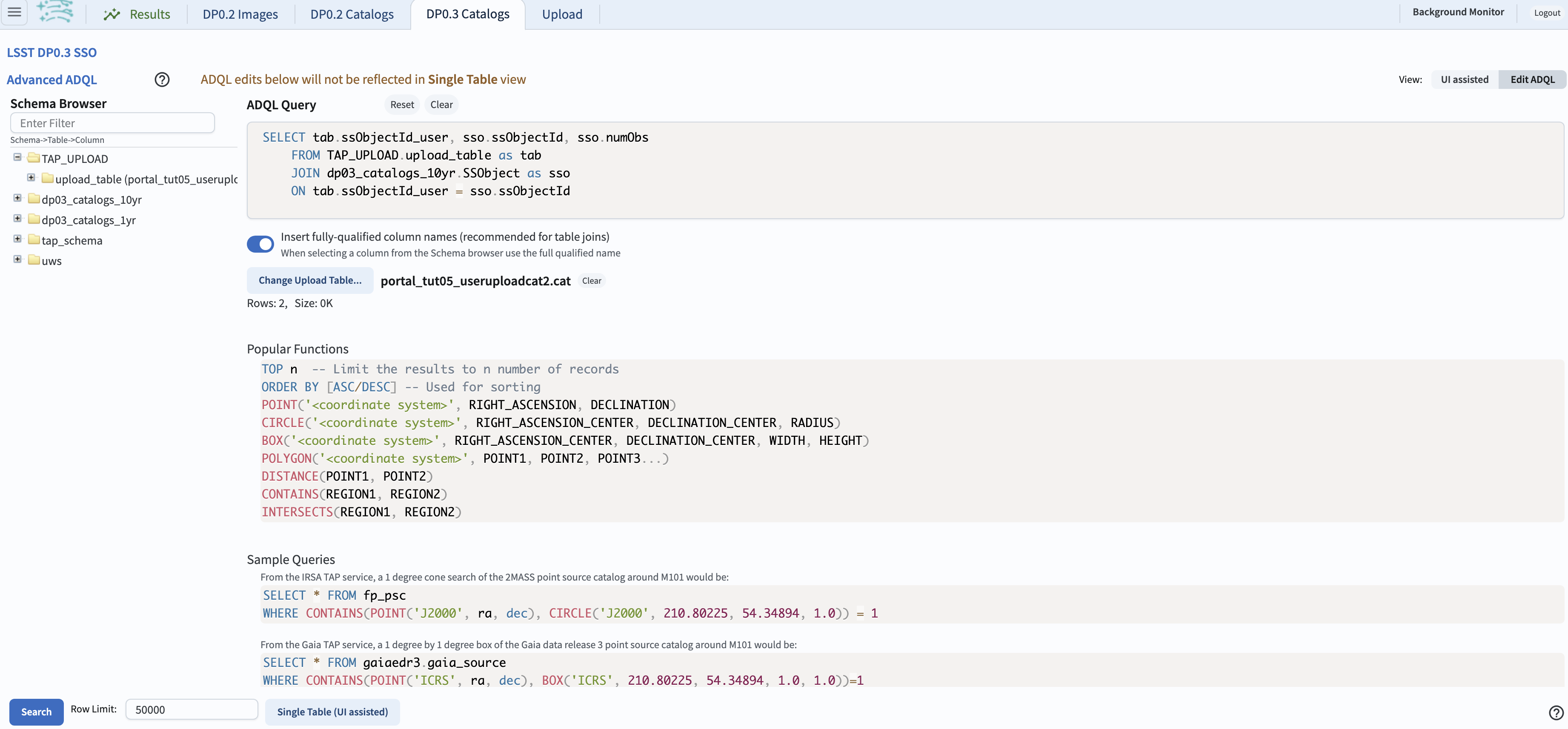
Figure 7: A screenshot of the portal user interface, ready to issue the query in the ADQL box.#
Step 3. Two-step search process using the “Loaded Table” option#
This section demonstrates a capability of the portal that enables analysis using multiple or more complex searches that are based on existing search results.
3.1. Return to the main DP0.3 Catalogs tab to go back to the search interface, and hit the “Reset Column Selections & Constraints” button on the top right. Also clear the previously uploaded table, by clicking the “Change Upload Table” button and in the pop-up window, click the “Clear File” gray button on the right. Make sure the Table Collection is still dp03_catalogs_10yr and the table is dp03_catalogs_10yr.DiaSource.
3.1a. As of Oct 22, 2024, a known bug in the portal does not completely clear the user uploaded table. In the meantime, the recommended workaround is to log out of the portal and log back in and repeat step 3.1.
3.2 In the Spatial section, enter some example coordinates (e.g. 314.9407129, -31.5520653 from the first table we uploaded in Section 1) and search the 10yr DiaSource catalog in a 100 arcsec radius cone, to retrieve a list of ssObjectIds. Make sure the “Spatial” box is checked and the “Temporal” box is unchecked. Click “Search”. Do not delete the search results (they will stay active), but go back to the main query UI page by clicking the “DP0.3 Catalogs” tab at the top.
If you recieve a search error “No coverage available” it is possible the uploaded tables were not properly cleared. Make sure you logged out of the portal and log back in and repeat step 3.1.
3.3. Then, go down to the Object ID Search section of the UI, and click the box to the left of Object ID Search, and click the arrow to expand the search options below. Click the “Load object IDs from a table” button which will lower a “Add Upload Table” button. Clicking that will open a new window to interface with loaded tables. Click the “Loaded Tables” tab at the top of the pop-up where a list of “tables” that are stored from recent searches is displayed. These will have a title labeled as the TAP catalog that was searched above (in this case, the example in step 3.1 searched the DiaSource catalog). The return of the search query can be identified as the earlier search from 3.1, since it will have the same number of rows returned (in this example, 110 DiaSources were returned). Click the “Load Table” button.
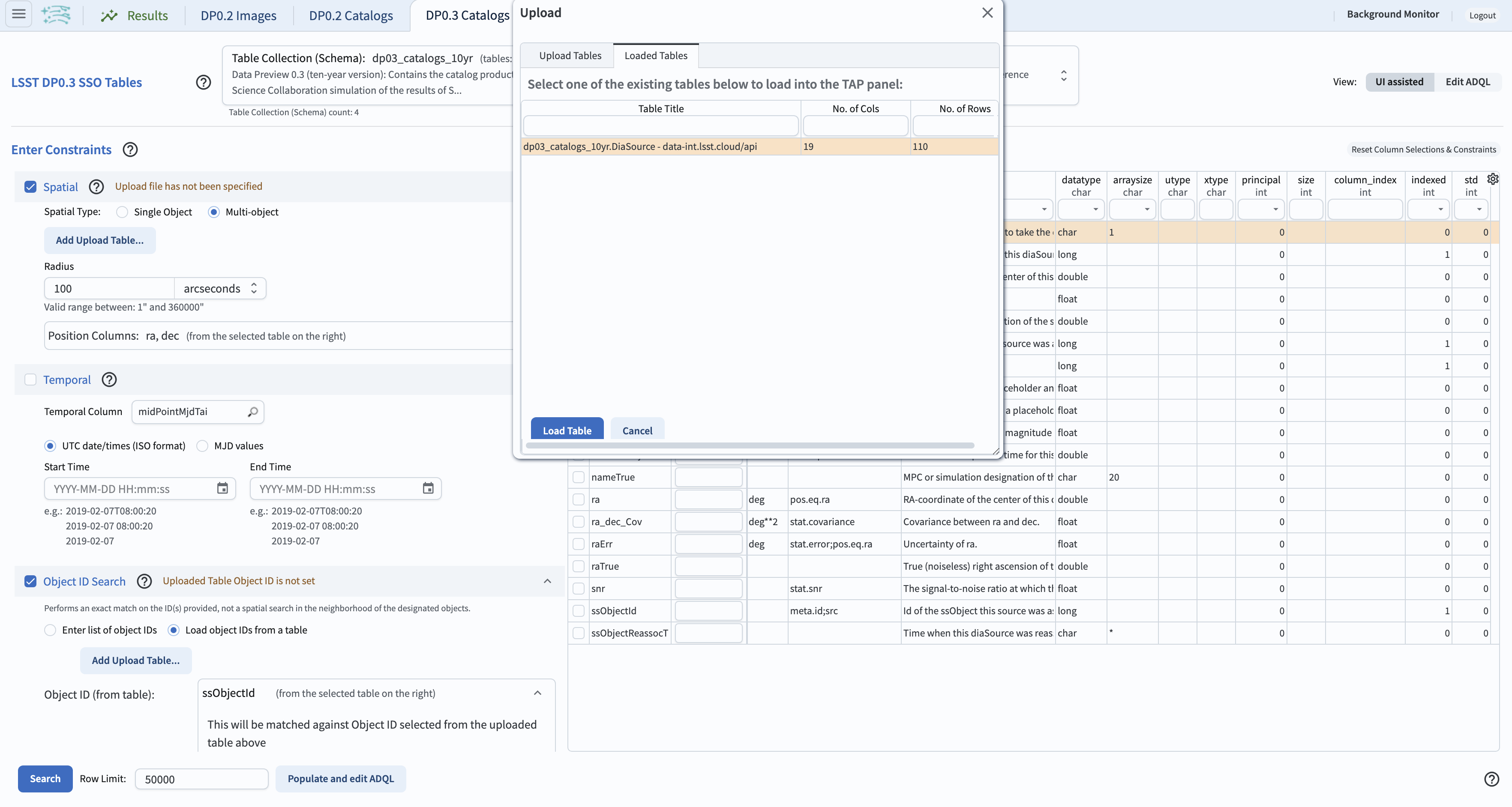
Figure 8: A screenshot of how to use the “Loaded Tables” option to access the previous query result.#
3.4. Click the magnifying glass next to the “Object ID” box to the right of where it says Uploaded Object ID (under the Change Upload Table button). Select the “ssObjectId” row and click “OK”, which loads the ssObjectId of the 110 returned entries from the search in Step 3.3.
3.5. Now in the panel labeled LSST DP0.3 SSO Tables at the top of the page, select the 10yr SSSource table. The Output Column Selection and Constraints table should update to reflect the column headers of the SSSource table. Back under Object ID search, where it says “Object ID (from table)” (in this case referring to the full DP0.3 table whose columns are listed on the right), click the magnifying glass and also select ssObjectId.
3.6. Click the magnifying glass next to “Object ID” box, now to the right of where it says “Object ID (from table):”. Again select the ssObjectId, which is what the parameter that will be matched on, click OK, and hit the Search button. The query will now search the SSSource table for all individual observations of objects which have these ssObjectIds from the query in 3.1. The query will return all SSSource observation entries for the list of 110 ssObjectIds. In this case, there are 19,077 individual observations of each of the 110 individual solar system bodies.
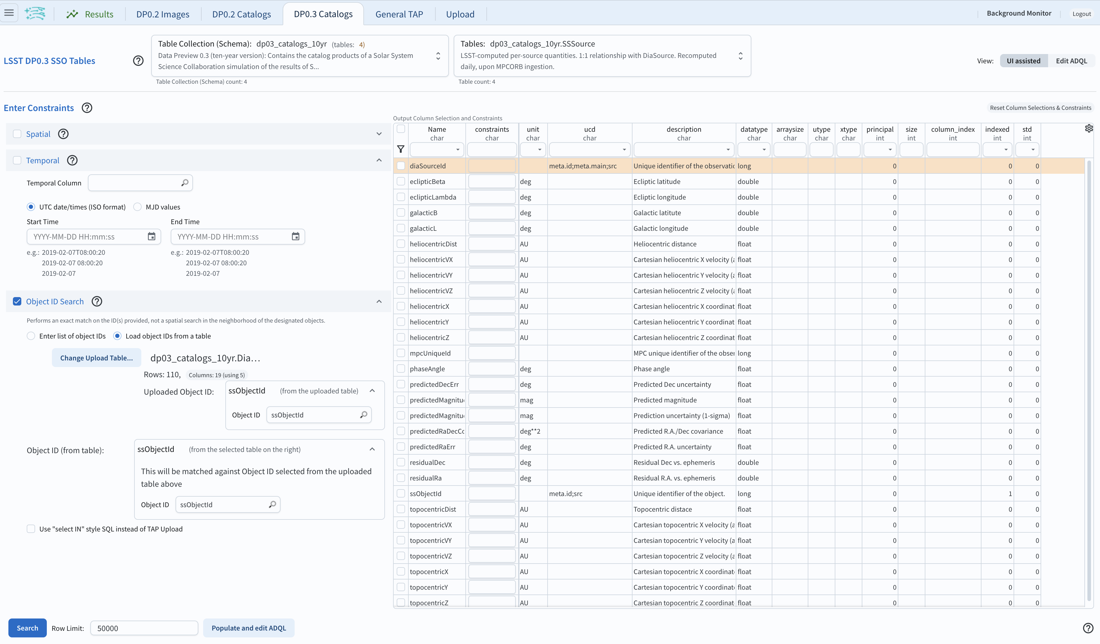
Figure 9: A screenshot of the fully populated “Object ID Search” section of the UI.#
3.7. By default the search results will create a scatter plot using the first two columns of the table. Modify the plot by clicking the single gear in the active chart panel, and select, for instance, helicentricY vs. heliocentricX as in the figure below. This plot shows the part of the orbit in heliocentric coordinates that is traced by the matched data of the solar system bodies during the 10 year survey data.
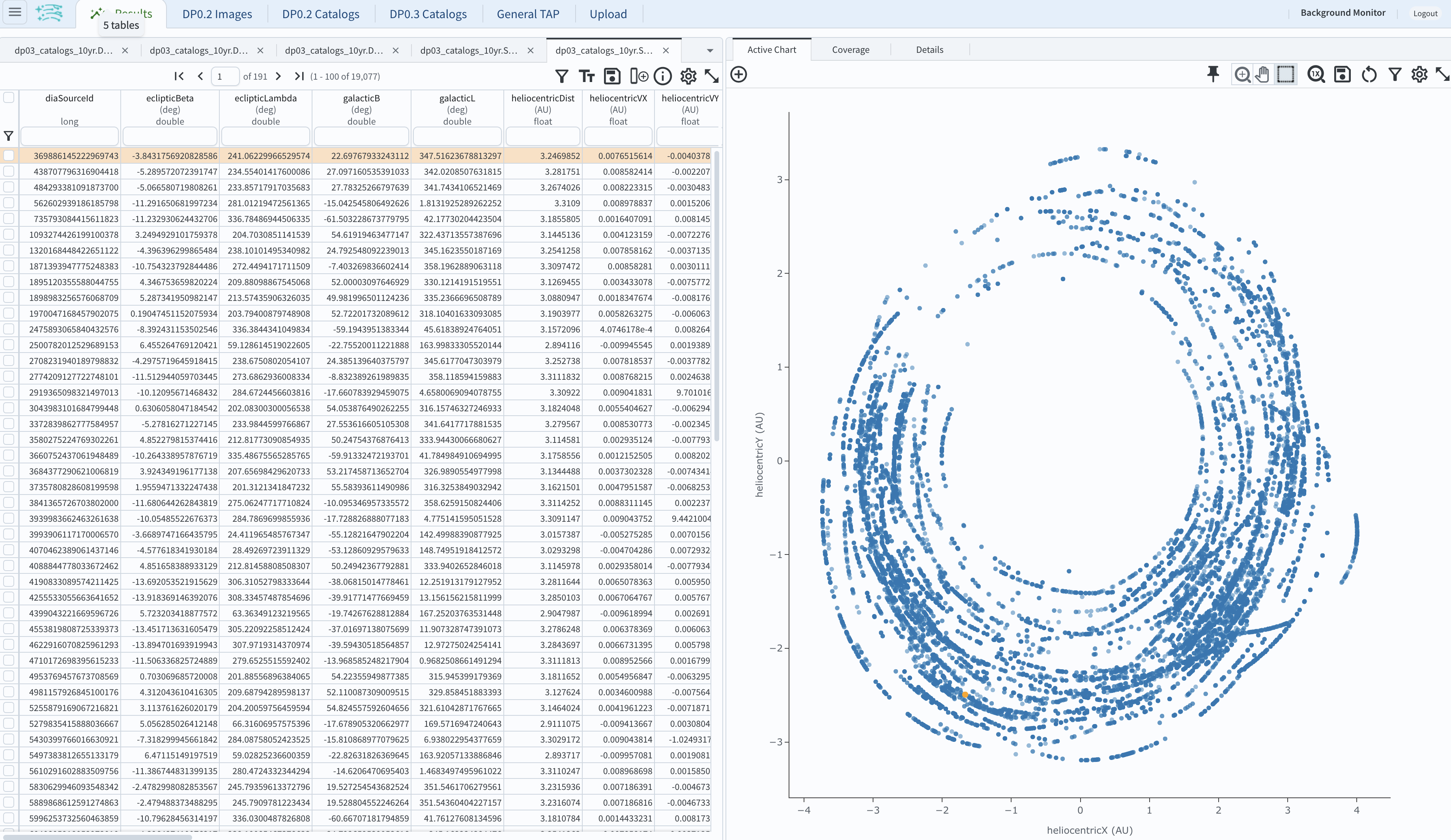
Figure 10: A screenshot showing the table resulting from your search, with the plot of helicentricY vs. heliocentricX.#
Step 4. Exercises for the learner#
4.1 Generate your own user table: perform a spatial and temporal search of the DiaSource table to look for a sample of solar system bodies observed in a specific part of the sky at a specific time. Save the query result table as a tsv, and use it to search the SSSource table for all observations that exist, by matching on ssObjectId.
4.2 Pick a favorite solar system object (for example, the first asteroid in the user uploaded table from step 2) and create a table that includes both the DiaSource table contents, and the SSSource table contents for the one object (with procedure similar to section 3 above). Note that after the first search, it is possible to select one row and remove the others using the “filter” option after the query completes.